library(astsa) # datos jj, globtemp
plot(jj, type = "o", ylab = "Quarterly Earnings per Share")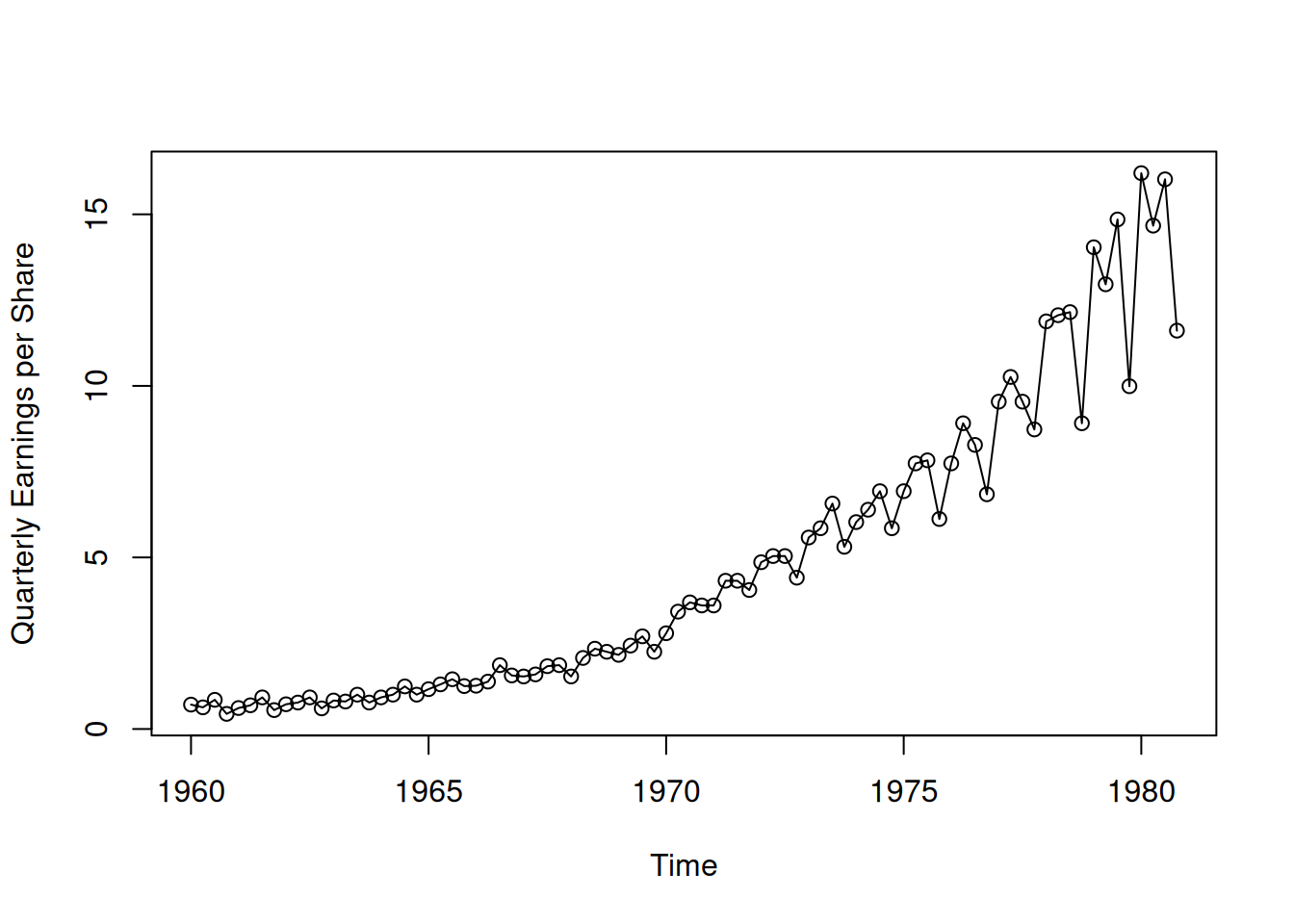
El objetivo es ilustrar, con series de tiempo reales, los patrones típicos y las preguntas estadísticas frecuentes que interesan a un analista. Varios casos:
Datos: \(n=84\) trimestres (21 años), de Q1-1960 a Q4-1980.
Patrones: tendencia creciente y estacionalidad trimestral marcada.
Enfoque típico: modelar \(y_t\) como
\[ y_t = \text{tendencia}_t + \text{estacionalidad}_{q(t)} + \varepsilon_t, \]
con \(q(t)\in\{1,2,3,4\}\), y evaluar su estructura (capítulos posteriores).
library(astsa) # datos jj, globtemp
plot(jj, type = "o", ylab = "Quarterly Earnings per Share")
O usando tidyverse:
# Paquetes
library(tidyverse)
── Attaching core tidyverse packages ──────────────────────── tidyverse 2.0.0 ──
✔ dplyr 1.1.4 ✔ readr 2.1.5
✔ forcats 1.0.0 ✔ stringr 1.5.2
✔ ggplot2 4.0.0 ✔ tibble 3.3.0
✔ lubridate 1.9.4 ✔ tidyr 1.3.1
✔ purrr 1.1.0
── Conflicts ────────────────────────────────────────── tidyverse_conflicts() ──
✖ dplyr::filter() masks stats::filter()
✖ dplyr::lag() masks stats::lag()
ℹ Use the conflicted package (<http://conflicted.r-lib.org/>) to force all conflicts to become errorslibrary(zoo) # as.yearqtr
Attaching package: 'zoo'

The following objects are masked from 'package:base':

as.Date, as.Date.numericlibrary(lubridate) # manejo de fechas
library(astsa)
# Convertir ts -> tibble con fecha trimestral
jj_tbl <- tibble(
date = as.Date(as.yearqtr(time(jj))), # Q1..Q4 a fecha (fin de trimestre)
eps = as.numeric(jj)
)
# Gráfico
jj_tbl %>%
ggplot(aes(date, eps)) +
geom_line() +
geom_point() +
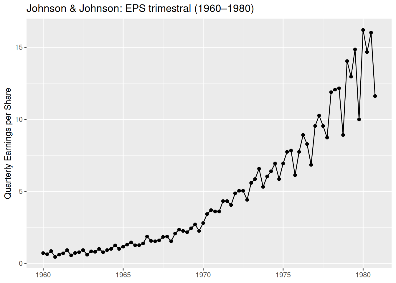
labs(
title = "Johnson & Johnson: EPS trimestral (1960–1980)",
x = NULL, y = "Quarterly Earnings per Share"
)
Datos: índice de temperatura media global tierra-océano (base 1951–1980, Hansen et al. [89] actualizado).
Variable: desviaciones en °C respecto a la media 1951–1980:
\[ T'_t = T_t - \bar{T}_{1951-1980} \]
Patrones observados:
Pregunta clave: ¿tendencia causada por procesos naturales o antropogénicos?
Observación: cambios porcentuales similares han ocurrido en escalas de 100 años (véase problema 2.8 con 634 años de sedimentos glaciares).
Interés principal: tendencia a largo plazo, no periodicidades.
Código R original (base R)
library(astsa)
plot(gtemp_both, type = "o", ylab = "Global Temperature Deviations")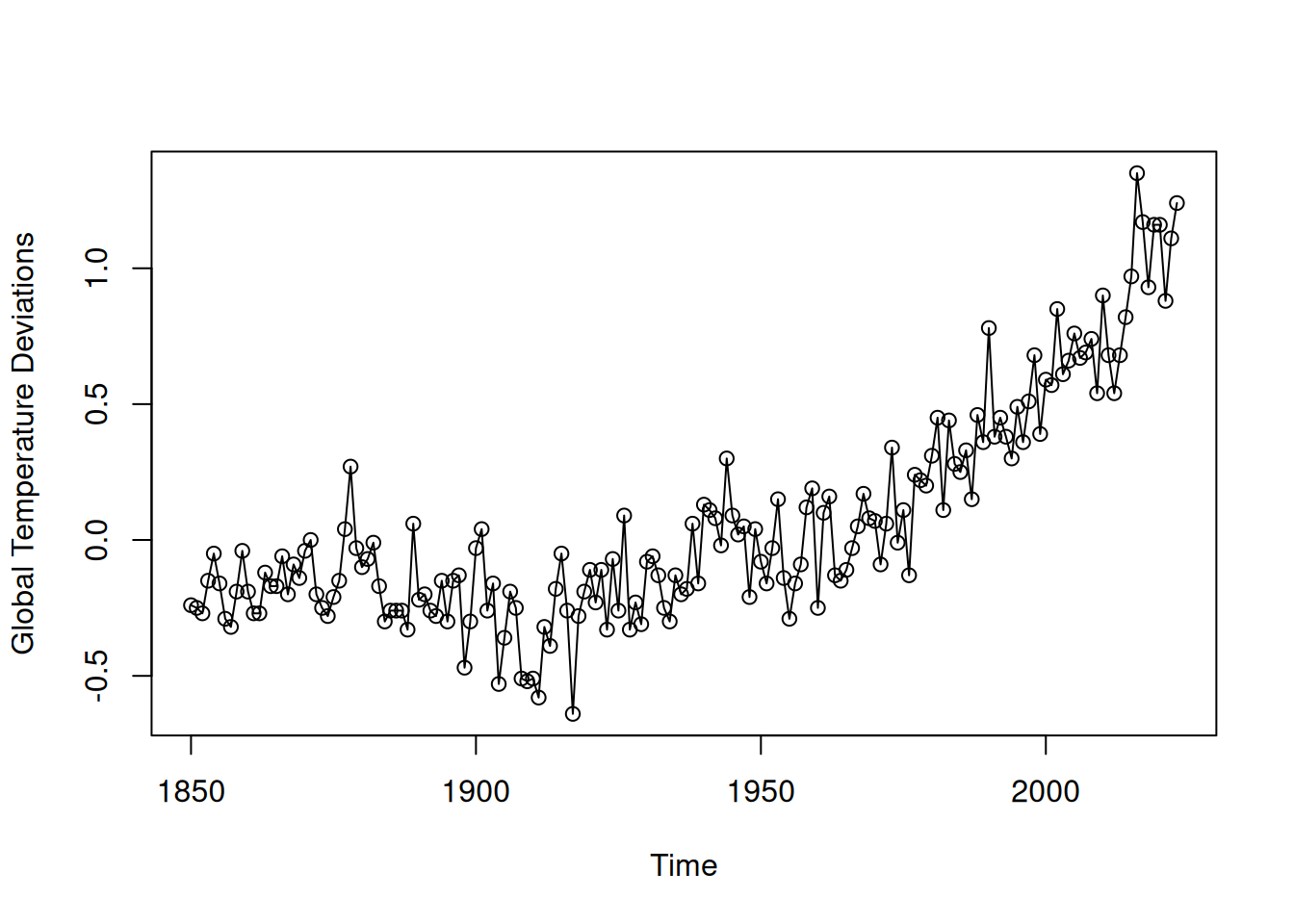
Usando tidyverse:
library(tidyverse)
library(astsa)
# Convertir ts -> tibble con año y desviación
gt_tbl <- tibble(
year = as.integer(floor(time(gtemp_both))),
temp_devC = as.numeric(gtemp_both)
)
# Gráfico con ggplot2
gt_tbl %>%
ggplot(aes(year, temp_devC)) +
geom_line() +
geom_point(size = 0.8) +
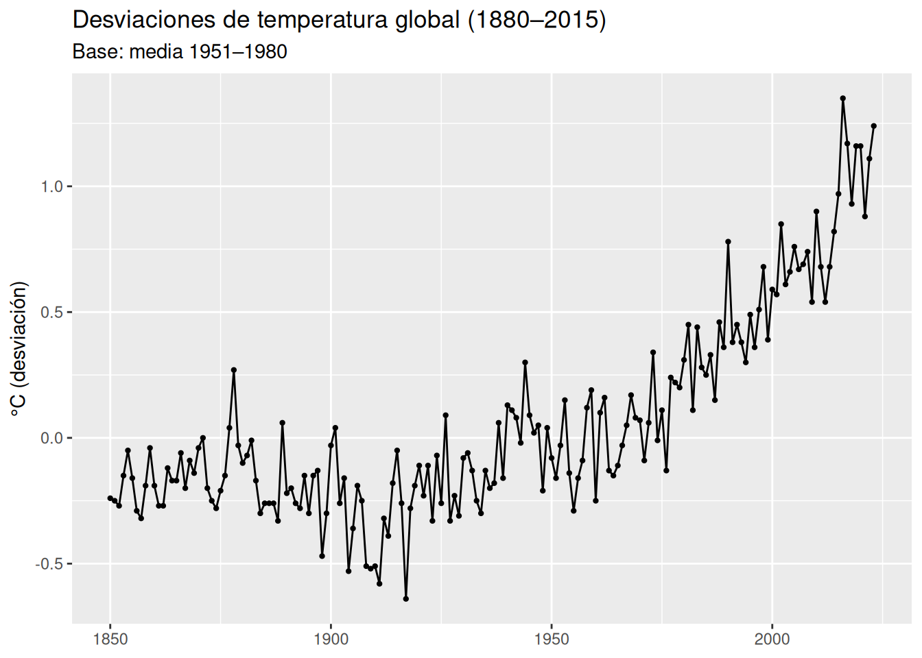
labs(
title = "Desviaciones de temperatura global (1880–2015)",
subtitle = "Base: media 1951–1980",
x = NULL, y = "°C (desviación)"
)
En términos generales, el análisis puede comenzar con un modelo aditivo simple:
\[ T'_t = \mu_t + \varepsilon_t \]
donde:
El objetivo inicial es estimar \(\mu_t\) y evaluar si el patrón observado es estadísticamente significativo y consistente con hipótesis de cambio climático.
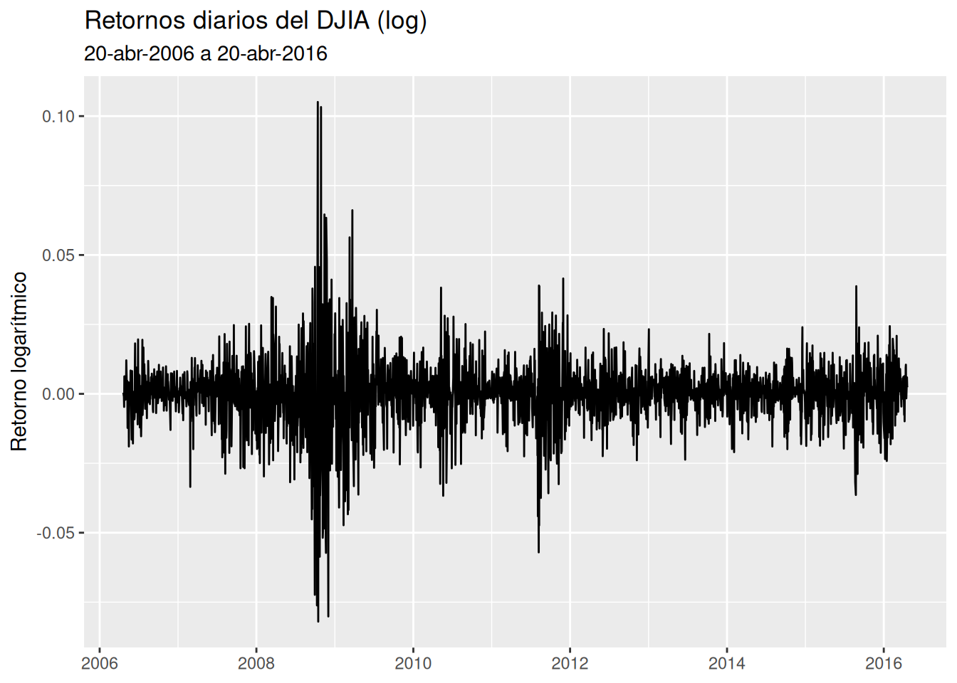
Datos: retornos diarios del DJIA del 20-abr-2006 al 20-abr-2016.
Fórmula del retorno:
\[ r_t = \frac{x_t - x_{t-1}}{x_{t-1}}, \quad 1+r_t = \frac{x_t}{x_{t-1}}, \]
y en forma logarítmica:
\[ \log(1+r_t) = \log(x_t) - \log(x_{t-1}) \approx r_t. \]
Características:
Problema típico: pronóstico de volatilidad.
Modelos relevantes: ARCH, GARCH (Engle, Bollerslev) y volatilidad estocástica (Harvey, Ruiz, Shephard).
Datos disponibles en astsa; para procesamiento se requiere xts.
Código R original (base R)
library(xts)
######################### Warning from 'xts' package ##########################
#                                                                             #
# The dplyr lag() function breaks how base R's lag() function is supposed to  #
# work, which breaks lag(my_xts). Calls to lag(my_xts) that you type or       #
# source() into this session won't work correctly.                            #
#                                                                             #
# Use stats::lag() to make sure you're not using dplyr::lag(), or you can add #
# conflictRules('dplyr', exclude = 'lag') to your .Rprofile to stop           #
# dplyr from breaking base R's lag() function.                                #
#                                                                             #
# Code in packages is not affected. It's protected by R's namespace mechanism #
# Set `options(xts.warn_dplyr_breaks_lag = FALSE)` to suppress this warning.  #
#                                                                             #
###############################################################################
Attaching package: 'xts'The following objects are masked from 'package:dplyr':
first, lastdjiar = diff(log(djia$Close))[-1] # retornos aproximados
plot(djiar, main = "DJIA Returns", type = "l")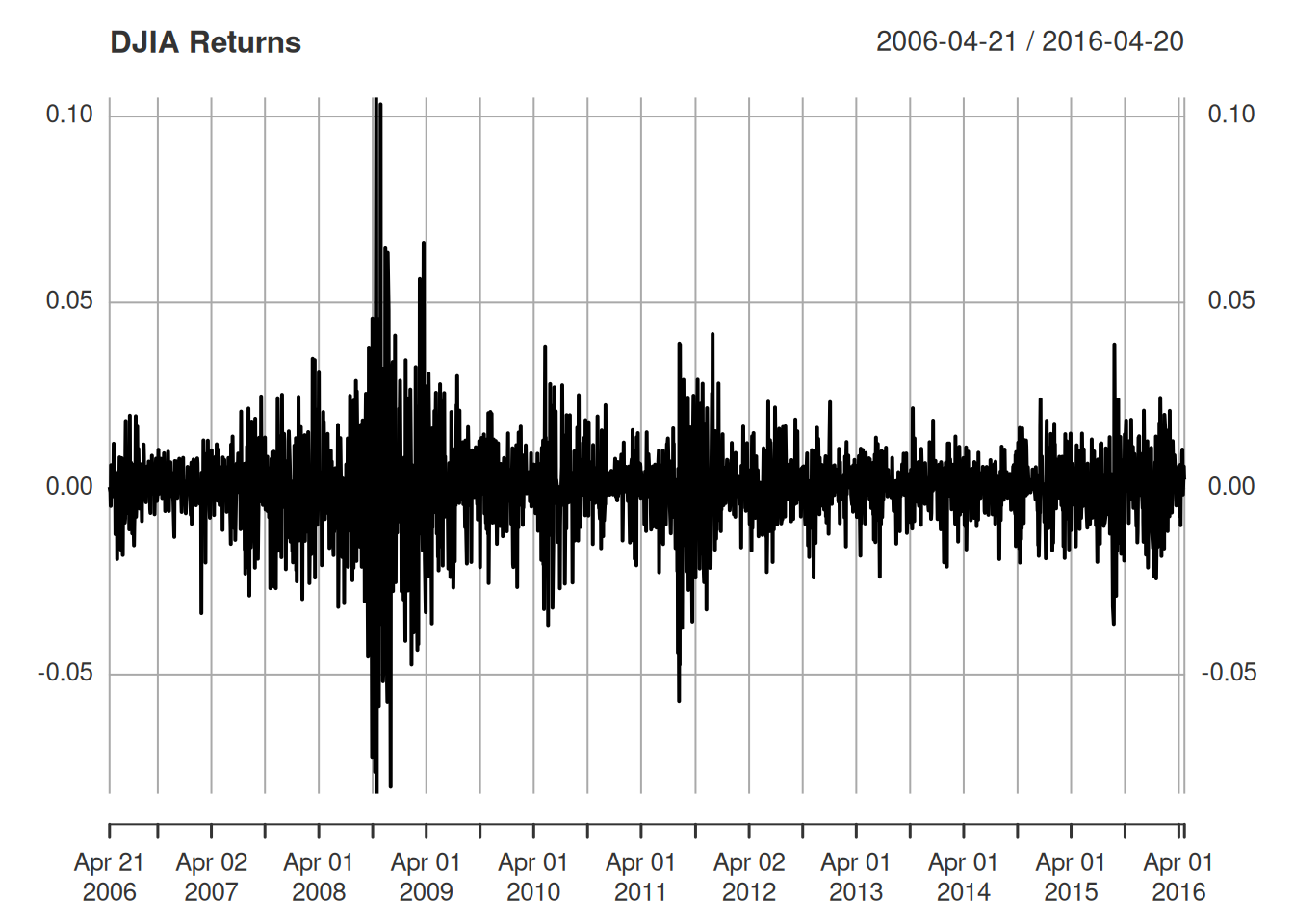
Código R en tidyverse
library(tidyverse)
library(astsa)   # datos djia
library(lubridate)

# Convertir a tibble con retornos logarítmicos
djia_tbl <- as_tibble(djia) %>%
  mutate(date = as.Date(index(djia))) %>%
  arrange(date) %>%
  mutate(
    log_ret = log(Close) - lag(log(Close))
  ) %>%
  filter(!is.na(log_ret))

# Gráfico de retornos
djia_tbl %>%
  ggplot(aes(date, log_ret)) +
  geom_line() +
  labs(
    title = "Retornos diarios del DJIA (log)",
    subtitle = "20-abr-2006 a 20-abr-2016",
    x = NULL, y = "Retorno logarítmico"
  )
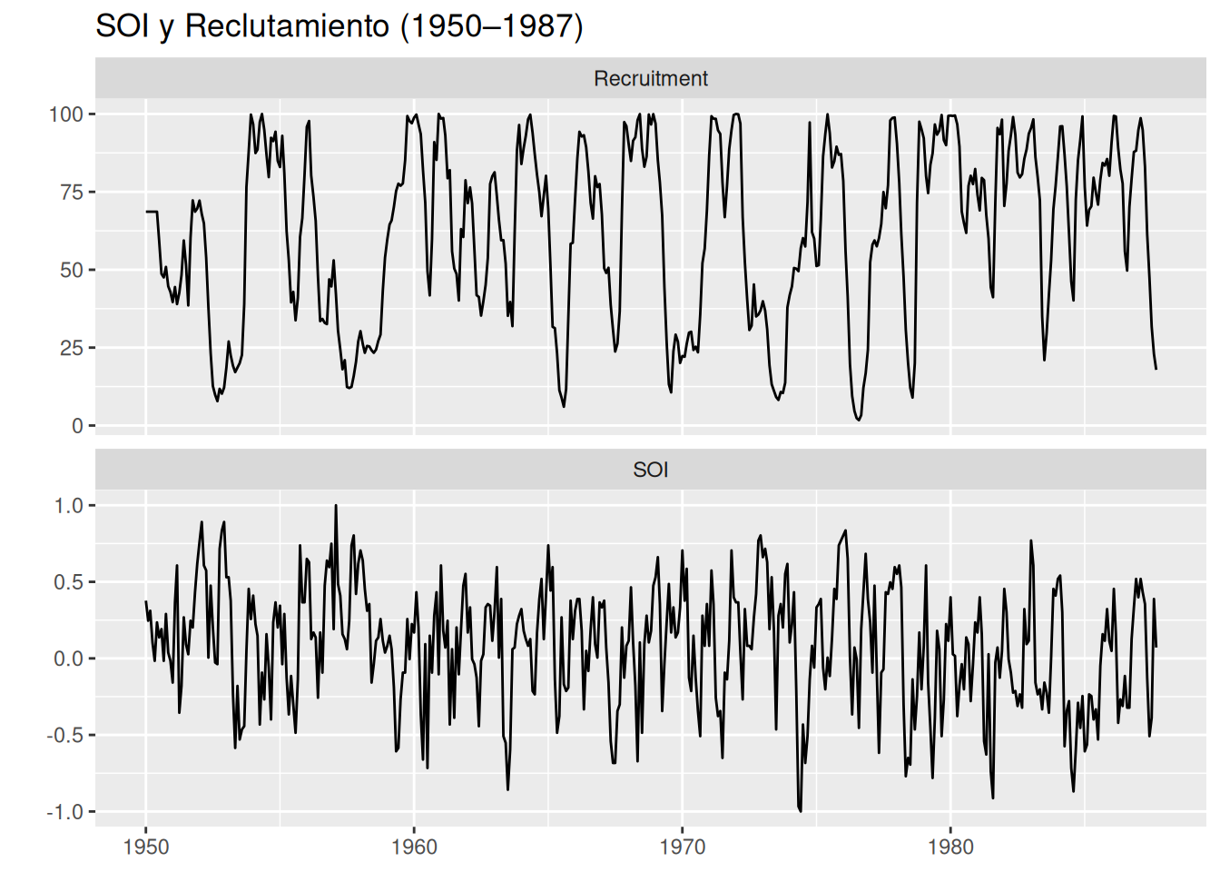
Datos mensuales:
Fenómenos:
El Niño: calentamiento cada 3–7 años en el Pacífico central.
Ciclos detectados:
Interés:
Identificar frecuencias dominantes en las series.
Analizar relación SOI–reclutamiento:
\[ \text{Recruitment}_t \; \text{vs} \; \text{SOI}_t \]
mediante regresión o modelos de función de transferencia.
Motivación: La temperatura oceánica puede influir en la dinámica de la población de peces.
Código R original (base R)
par(mfrow = c(2,1))
plot(soi, ylab = "", xlab = "", main = "Southern Oscillation Index")
plot(rec, ylab = "", xlab = "", main = "Recruitment")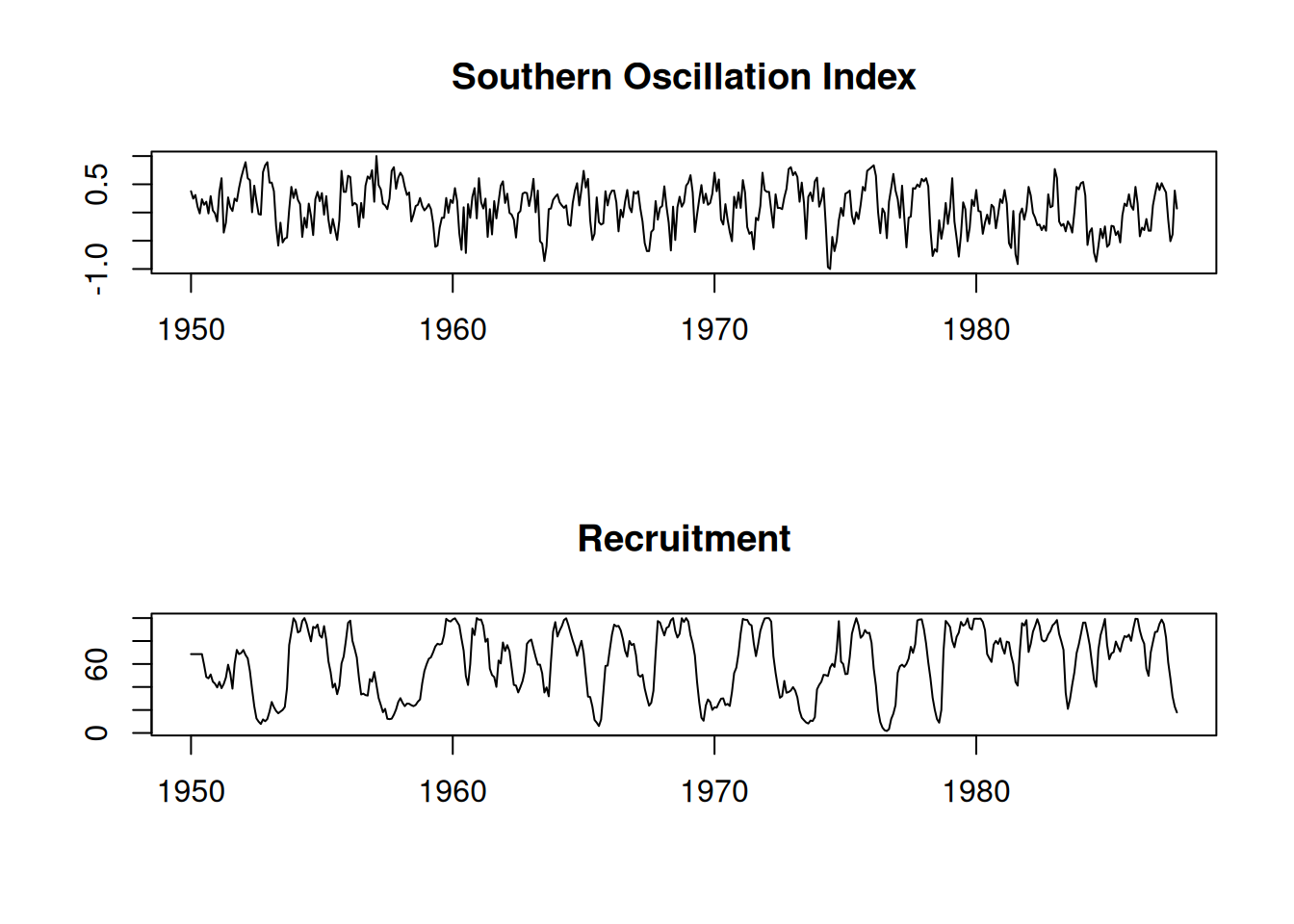
Código R en tidyverse
library(tidyverse)
library(astsa)  # datos soi y rec

# Conversión de ts a tibble
soi_tbl <- tibble(
  date = as.Date(time(soi)),
  SOI  = as.numeric(soi)
)

rec_tbl <- tibble(
  date = as.Date(time(rec)),
  Recruitment = as.numeric(rec)
)

# Graficar ambas series en paneles separados
bind_rows(
  soi_tbl %>% mutate(series = "SOI", value = SOI) %>% select(date, series, value),
  rec_tbl %>% mutate(series = "Recruitment", value = Recruitment) %>% select(date, series, value)
) %>%
  ggplot(aes(date, value)) +
  geom_line() +
  facet_wrap(~series, ncol = 1, scales = "free_y") +
  labs(
    title = "SOI y Reclutamiento (1950–1987)",
    x = NULL, y = ""
  )
Una serie de tiempo se modela como un conjunto de variables aleatorias ordenadas temporalmente:
\[ x_1, x_2, x_3, \dots \]
Conjunto genérico: \(\{x_t\}\), donde \(t\) es discreto (\(t = 0, \pm 1, \pm 2, \dots\)).
Realización: valores observados de un proceso estocástico.
Notación: se usa “serie de tiempo” para el proceso y su realización.
Representación gráfica:
Suavidad:
Diferencias en suavidad provienen de correlación serial:
\[ x_t \text{ depende de } x_{t-1}, x_{t-2}, \dots \]
set.seed(123)
w <- rnorm(500, 0, 1) %>% ts()

# Convertir a tibble para ggplot
w_df <- tibble(
  tiempo = seq_along(w),
  valor = as.numeric(w)
)

ggplot(w_df, aes(x = tiempo, y = valor)) +
  geom_line() +
  labs(title = "Ruido Blanco Gaussiano", x = "Tiempo", y = "Valor")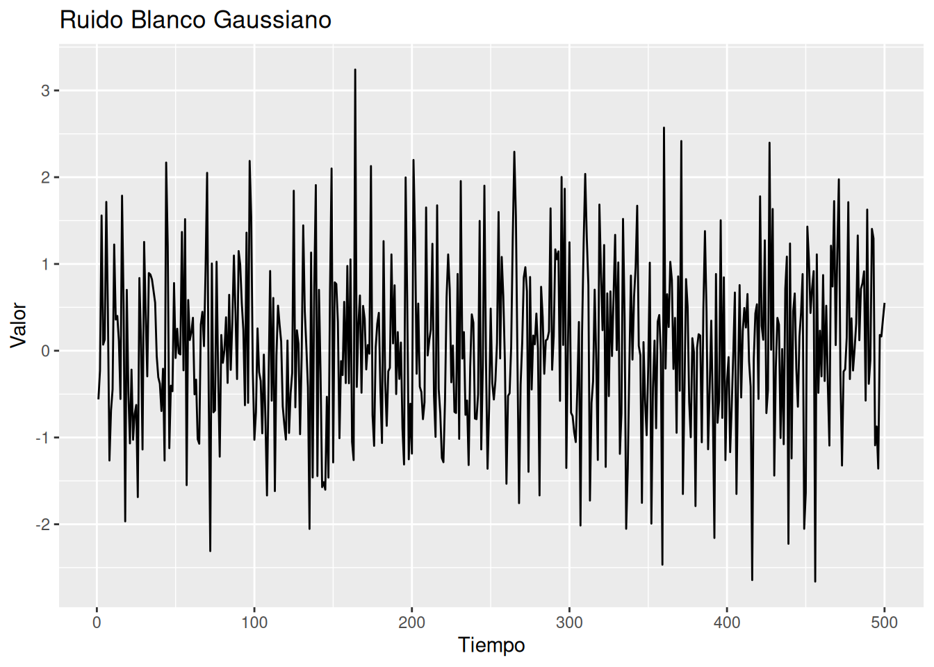
Promedio móvil simétrico:
\[ v_t = \frac{1}{3}(w_{t-1} + w_t + w_{t+1}) \]
Suaviza la serie, elimina oscilaciones rápidas.
w <- rnorm(500, 0, 1)

v <- stats::filter(w, sides = 2, filter = rep(1/3, 3))

# Convertir a tibble para graficar
v_df <- tibble(
  tiempo = seq_along(v),
  valor = as.numeric(v)
)

ggplot(v_df, aes(x = tiempo, y = valor)) +
  geom_line() +
  labs(title = "Promedio Móvil (3 puntos)", x = "Tiempo", y = "Valor")
Warning: Removed 2 rows containing missing values or values outside the scale range
(`geom_line()`).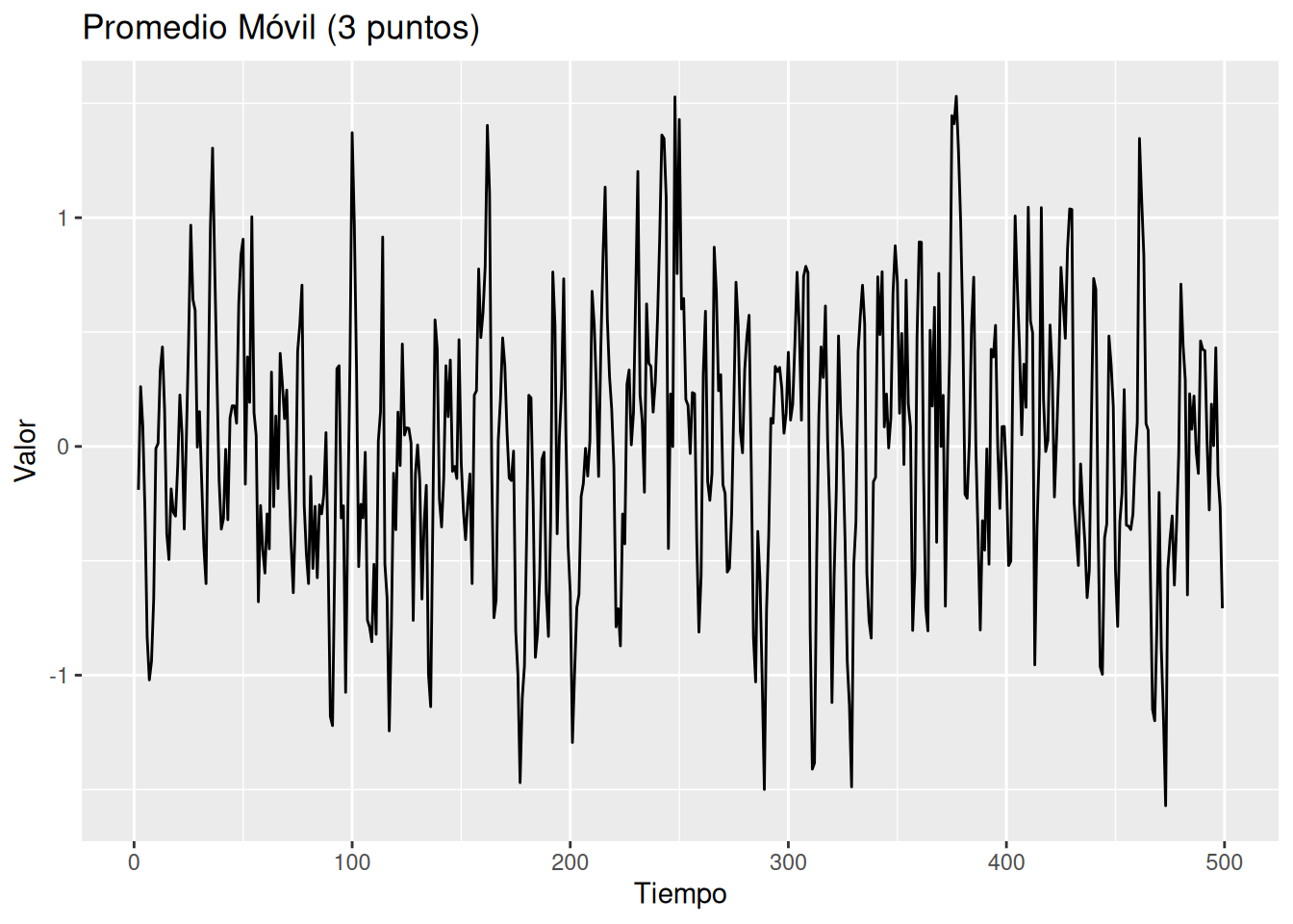
Modelo AR(2):
\[ x_t = x_{t-1} - 0.9 x_{t-2} + w_t \]
Genera comportamiento periódico.
w_ext <- rnorm(550, 0, 1)  # extra para “calentar” el filtro

x <- stats::filter(w_ext, filter = c(1, -0.9), method = "recursive")[-(1:50)]

ar_df <- tibble(
  tiempo = 1:500,
  x      = as.numeric(x)
)

ggplot(ar_df, aes(tiempo, x)) +
  geom_line() +
  labs(title = "AR(2): x_t = x_{t-1} - 0.9 x_{t-2} + w_t", x = "Tiempo", y = "x_t")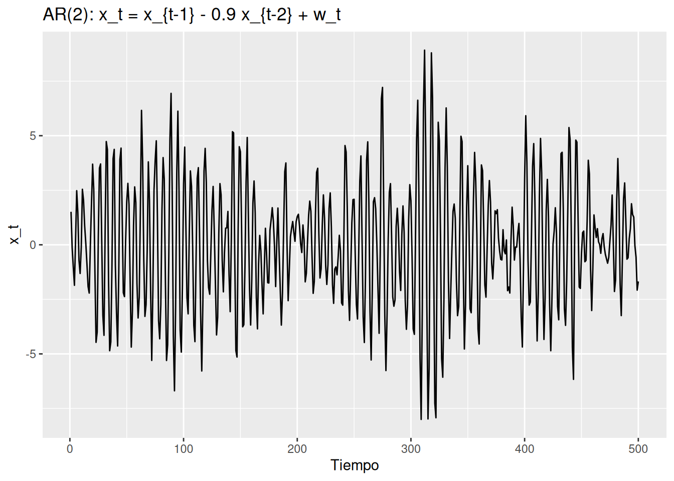
Modelo:
\[ x_t = \delta + x_{t-1} + w_t \]
Forma acumulada:
\[ x_t = \delta t + \sum_{j=1}^t w_j \]
set.seed(154)
w <- rnorm(200)
x <- cumsum(w)
xd <- cumsum(w + 0.2)

tibble(t = 1:200, sin_drift = x, con_drift = xd) %>%
  pivot_longer(-t) %>%
  ggplot(aes(t, value, color = name)) +
  geom_line() +
  geom_abline(intercept = 0, slope = 0.2, linetype = "dashed") +
  labs(title = "Caminata Aleatoria con y sin Deriva")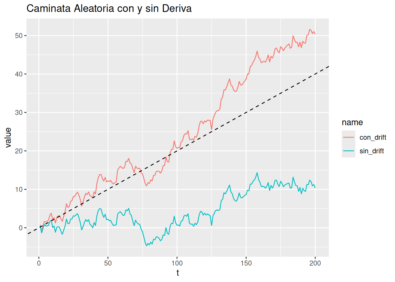
Modelo:
\[ x_t = 2 \cos\left( 2\pi \frac{t + 15}{50} \right) + w_t \]
Forma general:
\[ A\cos(2\pi \omega t + \phi) \]
donde \(A = 2\), \(\omega = 1/50\), \(\phi = 0.6\pi\).
Relación señal/ruido (SNR): mayor SNR → señal más detectable.
t <- 1:500
signal <- 2 * cos(2 * pi * t / 50 + 0.6 * pi)
w <- rnorm(500, 0, 1)

tibble(
  t,
  Señal = signal,
  SNR1 = signal + w,
  SNRbajo = signal + 5 * w
) %>%
  pivot_longer(-t) %>%
  ggplot(aes(t, value)) +
  geom_line() +
  facet_wrap(~name, scales = "free_y", ncol = 1)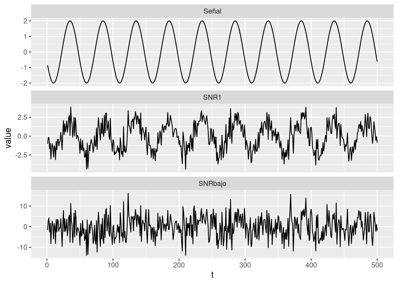
Forma:
\[ x_t = s_t + v_t \]
Aplicaciones: detección de señales, estimación de tendencias, componentes estacionales.
\[ F_{t_1, t_2, \ldots, t_n}(c_1, c_2, \ldots, c_n) = \Pr(x_{t_1} \leq c_1, \, x_{t_2} \leq c_2, \ldots, x_{t_n} \leq c_n) \]
Prácticamente difícil de trabajar salvo en el caso gaussiano.
Usualmente se analizan las marginales:
Definición:
\[ \mu_t = E(x_t) = \int_{-\infty}^\infty x f_t(x) dx \]
set.seed(123)

n <- 200
w <- rnorm(n)
v <- stats::filter(w, rep(1/3, 3), sides = 2)

tibble(t = 1:n, w = w, v = as.numeric(v)) %>%
  pivot_longer(-t, names_to = "serie", values_to = "valor") %>%
  ggplot(aes(t, valor, color = serie)) +
  geom_line() +
  geom_hline(yintercept = 0, linetype = "dashed")
Warning: Removed 2 rows containing missing values or values outside the scale range
(`geom_line()`).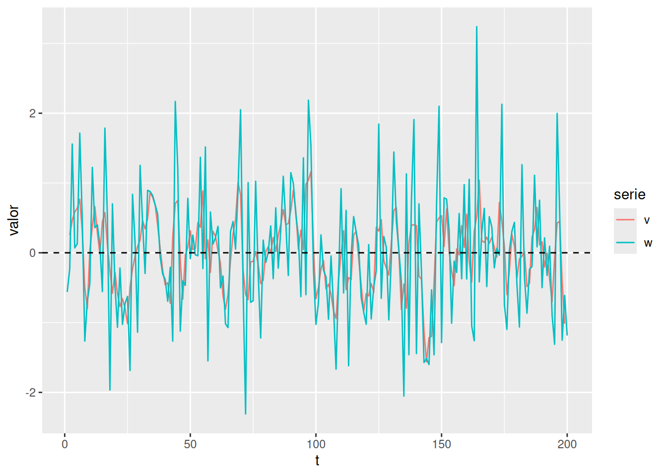
\[ x_t = \delta t + \sum_{j=1}^t w_j \]
delta <- 0.2
x <- cumsum(rnorm(n)) + delta*(1:n)
tibble(t = 1:n, x = x, mean_f = delta*(1:n)) %>%
  ggplot(aes(t, x)) +
  geom_line() +
  geom_line(aes(y = mean_f), color = "red", linetype = "dashed")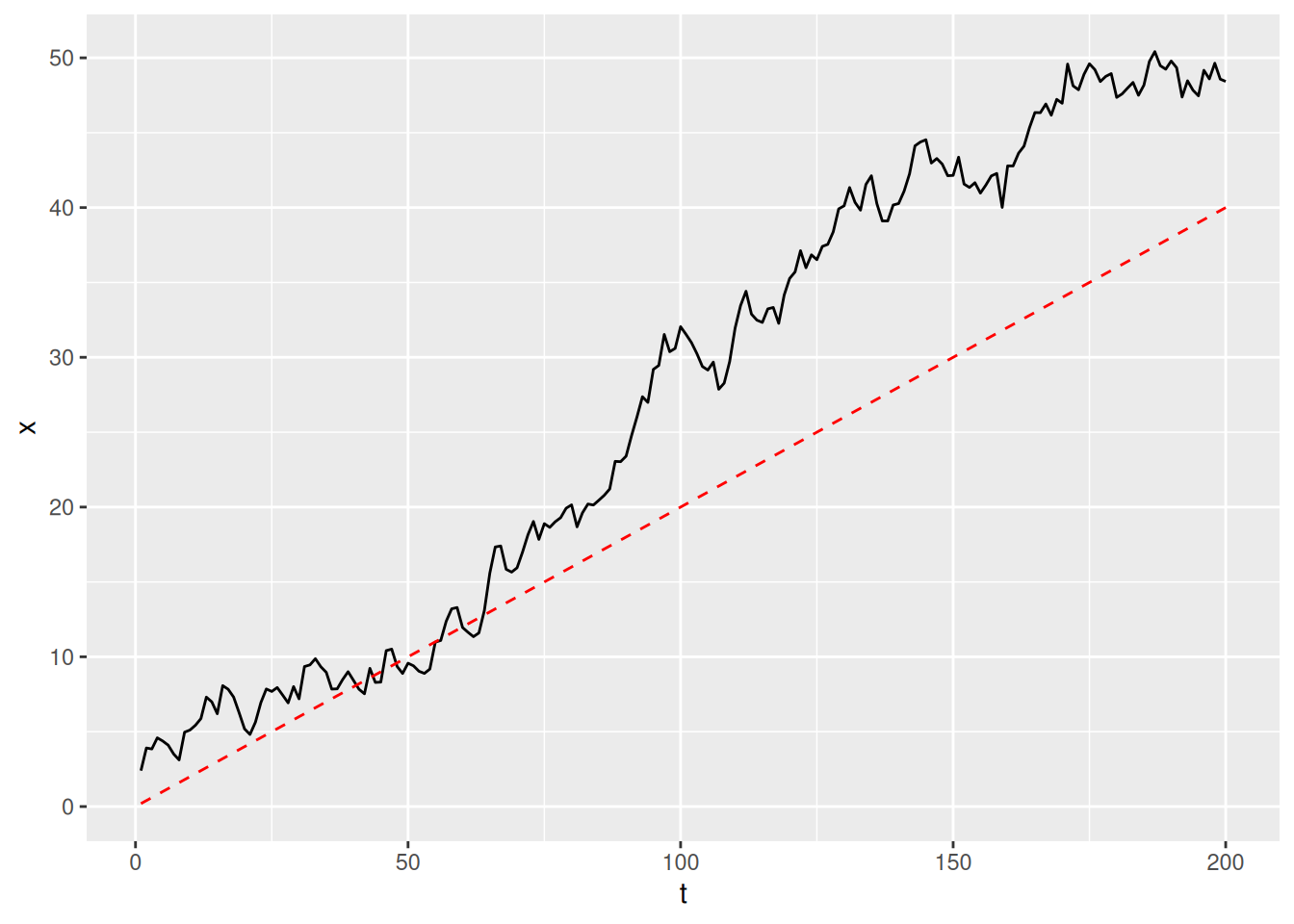
\[ x_t = 2 \cos\!\left(2\pi \tfrac{t+15}{50}\right) + w_t \]
signal <- 2*cos(2*pi*(1:n+15)/50)
x <- signal + rnorm(n)
tibble(t = 1:n, x = x, signal = signal) %>%
  ggplot(aes(t, x)) +
  geom_line() +
  geom_line(aes(y = signal), color = "blue", linetype = "dashed")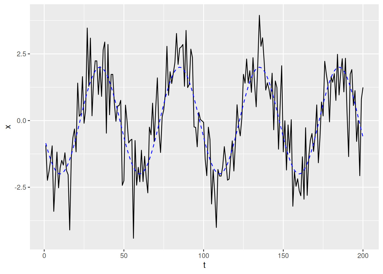
Definición:
\[ \gamma(s,t) = \text{cov}(x_s, x_t) = E[(x_s - \mu_s)(x_t - \mu_t)] \]
\[ \gamma_w(s,t) = \begin{cases} \sigma_w^2 & s=t \\ 0 & s \neq t \end{cases} \]
Propiedad: Combinaciones Lineales
Si \(U=\sum a_j X_j\), \(V=\sum b_k Y_k\) son combinaciones lineales de series \(X_j\) e \(Y_k\) con varianza finita entonces:
\[ \text{cov}(U,V) = \sum_{j,k} a_j b_k \text{cov}(X_j, Y_k) \]
\[ \gamma_v(s,t)= \begin{cases} \frac{3}{9}\sigma_w^2 & s=t \\ \frac{2}{9}\sigma_w^2 & |s-t|=1 \\ \frac{1}{9}\sigma_w^2 & |s-t|=2 \\ 0 & |s-t|>2 \end{cases} \]
\[ x_t = \sum_{j=1}^t w_j \]
Definición:
\[ \rho(s,t) = \frac{\gamma(s,t)}{\sqrt{\gamma(s,s)\gamma(t,t)}} \]
Definición:
\[ \gamma_{xy}(s,t) = E[(x_s - \mu_{xs})(y_t - \mu_{yt})] \]
Definición:
\[ \rho_{xy}(s,t) = \frac{\gamma_{xy}(s,t)}{\sqrt{\gamma_x(s,s)\gamma_y(t,t)}} \]
Para el caso en donde tenemos \(r\) series:
\[ \gamma_{jk}(s,t) = E[(x_{sj} - \mu_{sj})(x_{tk} - \mu_{tk})], \quad j,k=1,\ldots,r \]
Notas:
Una serie \(\{x_t\}\) es estrictamente estacionaria si, para todo \(k\), cualquier conjunto de tiempos \(t_1, \dots, t_k\), cualquier conjunto de constantes \(c_1, \dots, c_k\), y cualquier corrimiento \(h\), se cumple:
\[ \Pr\{x_{t_1} \leq c_1, \dots, x_{t_k} \leq c_k\} = \Pr\{x_{t_1+h} \leq c_1, \dots, x_{t_k+h} \leq c_k\} \]
Casos particulares - \(k=1\):
\[
\Pr\{x_s \leq c\} = \Pr\{x_t \leq c\}
\] \(\implies\) La media \(\mu_t\) debe ser constante en \(t\).
Es decir, depende solo de la diferencia de tiempos.
Una serie \(\{x_t\}\) es débilmente estacionaria si:
En lo sucesivo, estacionaria se refiere a este caso.
Notación simplificada - Media: \[ \mu_t = \mu \] - Autocovarianza: \[ \gamma(h) = \mathrm{Cov}(x_{t+h}, x_t) = \mathbb{E}[(x_{t+h}-\mu)(x_t-\mu)] \] - Autocorrelación: \[ \rho(h) = \frac{\gamma(h)}{\gamma(0)} \]
Con \(-1 \leq \rho(h) \leq 1\).
\(\implies\) Estacionario débil.
Si además es normal, también es estrictamente estacionario: \(\rho_w(0)=1\), \(\rho_w(h)=0\) si \(h \neq 0\).
\(\mu_{vt}=0\)
\(\gamma_v(h)= \begin{cases} \frac{3}{9}\sigma_w^2 & h=0 \\ \frac{2}{9}\sigma_w^2 & h=\pm 1 \\ \frac{1}{9}\sigma_w^2 & h=\pm 2 \\ 0 & |h|>2 \end{cases}\)
\(\rho_v(h)= \begin{cases} 1 & h=0 \\ 2/3 & h=\pm 1 \\ 1/3 & h=\pm 2 \\ 0 & |h|>2 \end{cases}\)
\(\implies\) No estacionaria.
\(\implies\) No estacionaria en media, pero sí en la covarianza.
Se llama tendencia estacionaria.
No negatividad: \[ 0 \leq \operatorname{Var}(a_1x_1+\dots+a_nx_n) = \sum_{j=1}^n \sum_{k=1}^n a_j a_k \gamma(j-k) \]
Varianza: \[ \gamma(0)=\mathbb{E}[(x_t-\mu)^2] \]
Acotamiento: \[ |\gamma(h)| \leq \gamma(0) \]
Simetría: \[ \gamma(h)=\gamma(-h) \]
Dos series \(x_t\) y \(y_t\) son conjuntamente estacionarias si cada una es estacionaria y:
Función de covarianza cruzada: \[ \gamma_{xy}(h)=\operatorname{Cov}(x_{t+h}, y_t) \]
Función de correlación cruzada (CCF): \[ \rho_{xy}(h)=\frac{\gamma_{xy}(h)}{\sqrt{\gamma_x(0)\gamma_y(0)}} \]
Propiedades:
Con \(x_t = w_t+w_{t-1}\) y \(y_t = w_t-w_{t-1}\):
Entonces: \[ \rho_{xy}(h)= \begin{cases} 0 & h=0 \\ 1/2 & h=1 \\ -1/2 & h=-1 \\ 0 & |h|\geq 2 \end{cases} \]
\(\implies\) \(x_t\) y \(y_t\) son conjuntamente estacionarias.
Si \(y_t = A x_{t-\ell} + w_t\) entonces \(x_t\) lidera a \(y_t\) si \(\ell>0\) y rezaga a \(y_t\) si \(\ell<0\).
Cálculo: \[ \gamma_{yx}(h) = A \gamma_x(h-\ell) \]
Se observa un pico en \(\gamma_{yx}(h)\) en \(h=\ell\).
Ejemplo en R
library(dplyr)

set.seed(123)
x <- rnorm(100)
y <- stats::lag(x, -5) + rnorm(100)

ccf(x, y, ylab = "CCovF", type = "covariance")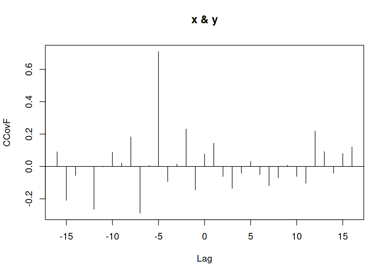
Definición:
\[ x_t = \mu + \sum_{j=-\infty}^\infty \psi_j w_{t-j}, \quad \sum_{j=-\infty}^\infty |\psi_j| < \infty \]
Autocovarianza:
\[ \gamma_x(h) = \sigma_w^2 \sum_{j=-\infty}^\infty \psi_{j+h}\psi_j \]
Definición: \({x_t}\) es Gaussiano si para cualquier conjunto de tiempos \(t_1,\dots,t_n\), el vector \((x_{t_1}, \dots, x_{t_n})'\) es multinormal con densidad:
\[ f(x)=(2\pi)^{-n/2}|\Gamma|^{-1/2}\exp\left\{-\tfrac{1}{2}(x-\mu)'\Gamma^{-1}(x-\mu)\right\} \]
Para una serie estacionaria, \(\mu_t = \mu\) es constante y puede estimarse con:
\[ \bar{x} = \frac{1}{n} \sum_{t=1}^n x_t \]
Varianza del estimador:
\[ \operatorname{var}(\bar{x}) = \frac{1}{n} \sum_{h=-n}^n \left(1-\frac{|h|}{n}\right) \gamma_x(h) \]
Definición Autocovarianza muestral:
\[ \hat{\gamma}(h) = n^{-1} \sum_{t=1}^{n-h} (x_{t+h}-\bar{x})(x_t-\bar{x}), \quad \hat{\gamma}(-h)=\hat{\gamma}(h) \]
Definición Autocorrelación muestral:
\[ \hat{\rho}(h) = \frac{\hat{\gamma}(h)}{\hat{\gamma}(0)} \]
La estimación de \(\rho(h)\) se hace con pares \((x_t, x_{t+h})\). Ejemplo con la serie SOI:
r <- round(acf(soi, 6, plot=FALSE)$acf[-1], 3)
show(r)
[1] 0.604 0.374 0.214 0.050 -0.107 -0.187par(mfrow=c(1,2))
plot(stats::lag(soi, -1), soi); legend("topleft", legend=r[1])
plot(stats::lag(soi, -6), soi); legend("topleft", legend=r[6])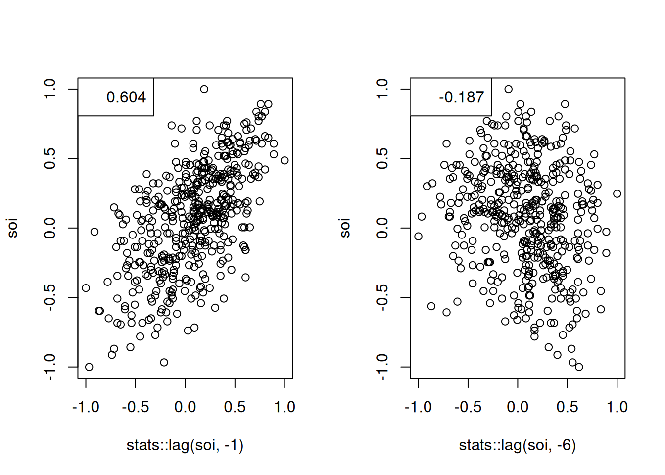
Propiedad Distribución asintótica de la ACF
Si \(x_t\) es ruido blanco y \(n\) es grande:
\[ \hat{\rho}_x(h) \sim N(0, 1/n), \quad h=1,2,\dots,H \]
Criterio práctico: \(\hat{\rho}(h)\) es significativo si está fuera de \(\pm 2/\sqrt{n}\).
Modelo:
\[ y_t = 5 + x_t - 0.7 x_{t-1}, \quad x_t \in \{-1,1\} \]
Comparación con \(n=10\) y \(n=100\).
set.seed(101010)
x1 <- 2*rbinom(11, 1, .5) - 1
x2 <- 2*rbinom(101, 1, .5) - 1
y1 <- 5 + stats::filter(x1, sides=1, filter=c(1,-.7))[-1]
y2 <- 5 + stats::filter(x2, sides=1, filter=c(1,-.7))[-1]

plot.ts(y1, type="s")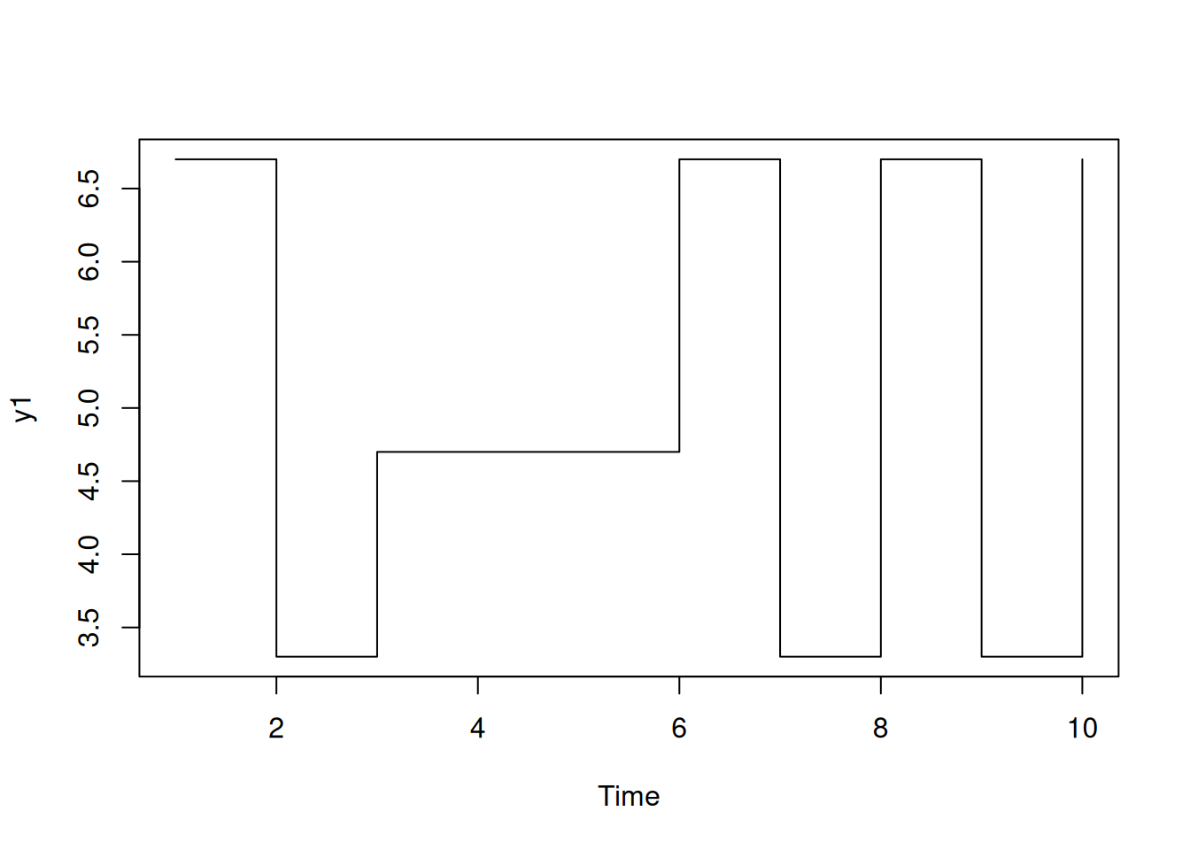
plot.ts(y2, type="s")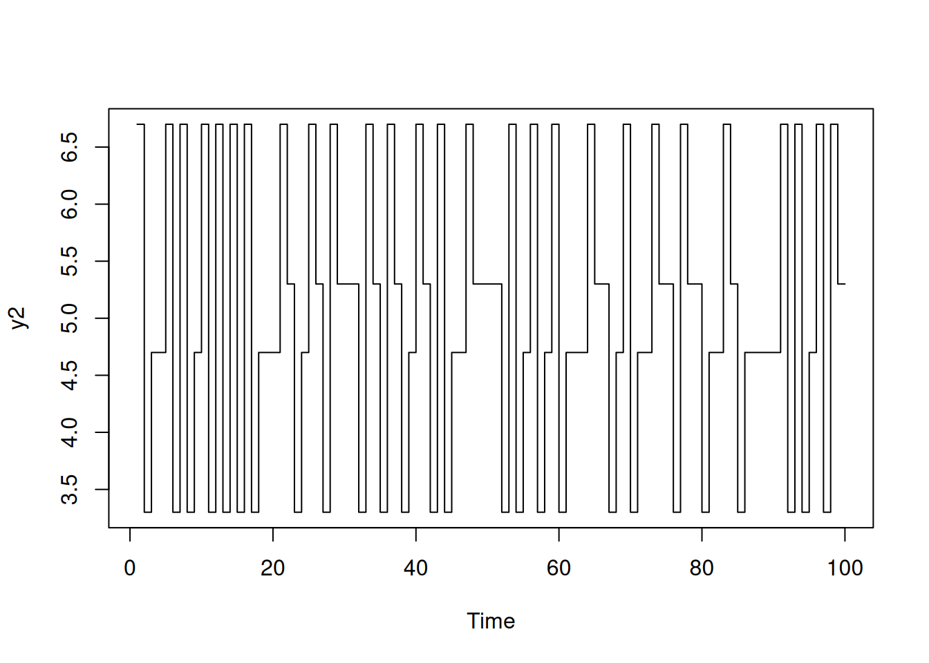
c(mean(y1), mean(y2))[1] 5.080 5.002acf(y1, lag.max=4, plot=FALSE)
Autocorrelations of series 'y1', by lag

     0      1      2      3      4
1.000 -0.688 0.425 -0.306 -0.007 acf(y2, lag.max=4, plot=FALSE)
Autocorrelations of series 'y2', by lag

     0      1      2      3      4
 1.000 -0.480 -0.002 -0.004  0.000
Teóricamente:
\[ \rho_y(1) = \frac{-0.7}{1+0.7^2} = -0.47, \quad \rho_y(h)=0 \text{ si } |h|>1 \]
Definición Covarianza cruzada muestral:
\[ \hat{\gamma}_{xy}(h) = n^{-1} \sum_{t=1}^{n-h} (x_{t+h}-\bar{x})(y_t-\bar{y}), \quad \hat{\gamma}_{xy}(-h)=\hat{\gamma}_{yx}(h) \]
Definición Correlación cruzada muestral:
\[ \hat{\rho}_{xy}(h) = \frac{\hat{\gamma}_{xy}(h)}{\sqrt{\hat{\gamma}_x(0)\hat{\gamma}_y(0)}} \]
Propiedad Distribución asintótica de la correlación cruzada
Si uno de los procesos es ruido blanco:
\[ \hat{\rho}_{xy}(h) \sim N(0, 1/n) \]
par(mfrow=c(3,1))
acf(soi, 48, main="Southern Oscillation Index")
acf(rec, 48, main="Recruitment")
ccf(soi, rec, 48, main="SOI vs Recruitment", ylab="CCF")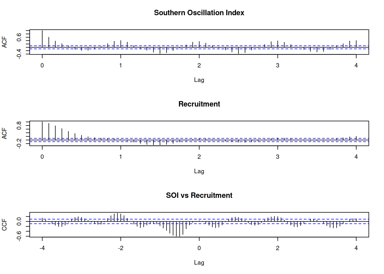
Generación de dos series independientes con comportamiento cíclico:
\[ x_t = 2\cos\left(2\pi t/12\right) + w_{t1}, \quad y_t = 2\cos\left(2\pi (t+5)/12\right) + w_{t2} \]
El preblanqueo elimina la señal de \(y_t\) ajustando regresión con \(\cos\) y \(\sin\).
set.seed(1492)
num <- 120; t <- 1:num
X <- ts(2*cos(2*pi*t/12) + rnorm(num), freq=12)
Y <- ts(2*cos(2*pi*(t+5)/12) + rnorm(num), freq=12)

Yw <- resid(lm(Y ~ cos(2*pi*t/12) + sin(2*pi*t/12), na.action=NULL))

par(mfrow=c(3,2), mgp=c(1.6,.6,0), mar=c(3,3,1,1))
plot(X); plot(Y)
acf(X,48, ylab="ACF(X)")
acf(Y,48, ylab="ACF(Y)")
ccf(X,Y,24, ylab="CCF(X,Y)")
ccf(X,Yw,24, ylab="CCF(X,Yw)", ylim=c(-.6,.6))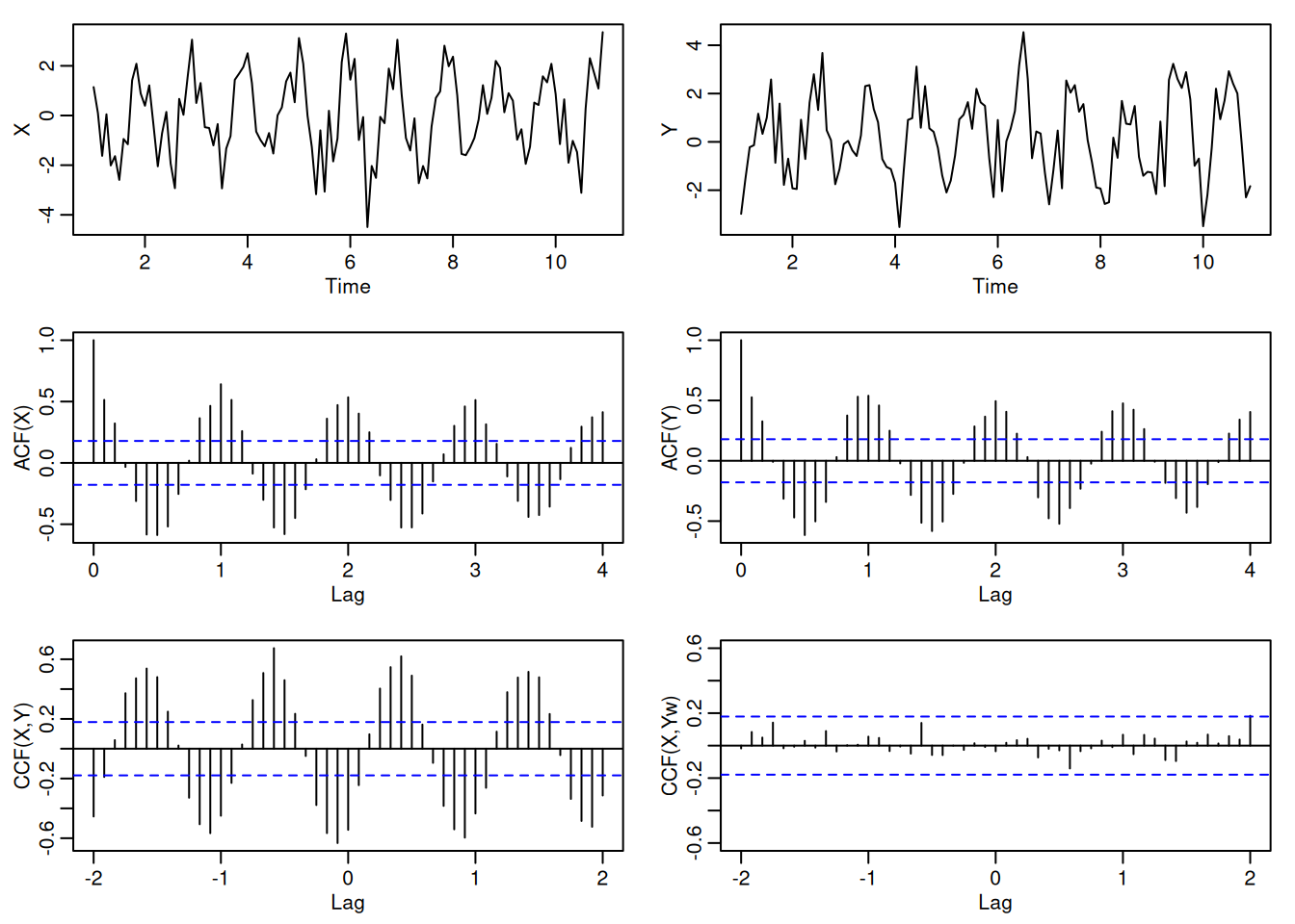
Sea \(x_t = (x_{t1}, x_{t2}, \ldots, x_{tp})'\) un vector de \(p\) series de tiempo.
\[ \mu = \mathbb{E}(x_t) \]
\[ \Gamma(h) = \mathbb{E}\left[(x_{t+h}-\mu)(x_t-\mu)'\right] \]
\[ \gamma_{ij}(h) = \mathbb{E}[(x_{t+h,i}-\mu_i)(x_{tj}-\mu_j)] \]
\[ \Gamma(-h) = \Gamma'(h) \]
\[ \hat{\Gamma}(h) = \frac{1}{n}\sum_{t=1}^{n-h} (x_{t+h}-\bar{x})(x_t-\bar{x})' \]
\[ \bar{x} = \frac{1}{n} \sum_{t=1}^n x_t \]
\[ \hat{\Gamma}(-h) = \hat{\Gamma}(h)' \]
Un proceso \(x_s\) puede estar indexado por un vector de coordenadas espaciales/temporales \(s=(s_1, s_2, \ldots, s_r)'\).
\[ \gamma(h) = \mathbb{E}[(x_{s+h}-\mu)(x_s-\mu)] \]
\[ \mu = \mathbb{E}(x_s) \]
En el caso bidimensional (\(r=2\)):
\[ \gamma(h_1,h_2) = \mathbb{E}[(x_{s_1+h_1,s_2+h_2}-\mu)(x_{s_1,s_2}-\mu)] \]
\[ \hat{\gamma}(h) = (S_1 S_2 \cdots S_r)^{-1} \sum_{s_1}\sum_{s_2}\cdots\sum_{s_r} (x_{s+h}-\bar{x})(x_s-\bar{x}) \]
\[ \bar{x} = (S_1 S_2 \cdots S_r)^{-1}\sum_{s_1}\sum_{s_2}\cdots\sum_{s_r} x_{s_1,s_2,\dots,s_r} \]
\[ \hat{\rho}(h) = \frac{\hat{\gamma}(h)}{\hat{\gamma}(0)} \]
Serie de temperaturas medidas en una grilla \(64 \times 36\). Se observa un cambio a partir de la fila 40, con oscilaciones más estables y periódicas.
Cálculo de promedios por fila:
persp(1:64, 1:36, soiltemp, phi=25, theta=25, scale=FALSE,
      expand=4, ticktype="detailed",
      xlab="rows", ylab="cols", zlab="temperature")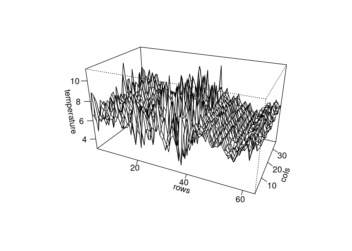
plot.ts(rowMeans(soiltemp), xlab="row", ylab="Average Temperature")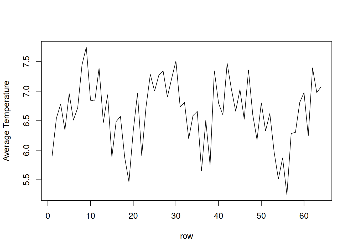
\[ \hat{\rho}(h_1,h_2) = \frac{\hat{\gamma}(h_1,h_2)}{\hat{\gamma}(0,0)} \]
con
\[ \hat{\gamma}(h_1,h_2) = (S_1 S_2)^{-1}\sum_{s_1}\sum_{s_2}(x_{s_1+h_1,s_2+h_2}-\bar{x})(x_{s_1,s_2}-\bar{x}) \]
fs <- Mod(fft(soiltemp - mean(soiltemp)))^2/(64*36)
cs <- Re(fft(fs, inverse=TRUE)/sqrt(64*36)) # ACovF
rs <- cs/cs[1,1] # ACF
rs2 <- cbind(rs[1:41,21:2], rs[1:41,1:21])
rs3 <- rbind(rs2[41:2,], rs2)

par(mar=c(1,2.5,0,0)+.1)
persp(-40:40, -20:20, rs3, phi=30, theta=30, expand=30, scale="FALSE",
      ticktype="detailed", xlab="row lags", ylab="column lags",
      zlab="ACF")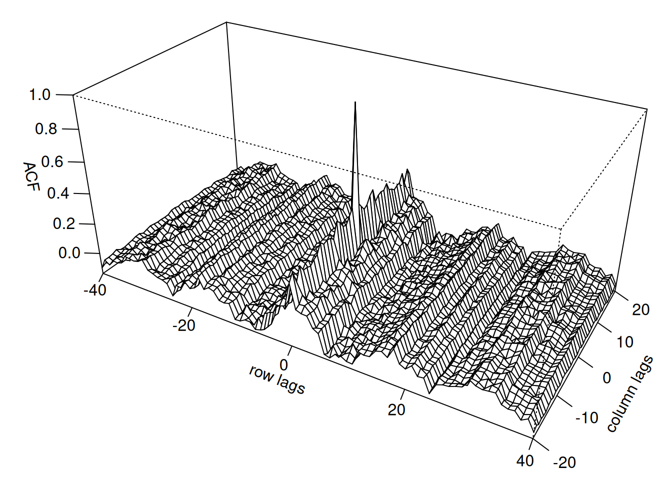
En casos de observaciones irregulares se utiliza el variograma:
\[ 2V_x(h) = \operatorname{Var}(x_{s+h}-x_s) \]
\[ 2\hat{V}_x(h) = \frac{1}{N(h)} \sum_s (x_{s+h}-x_s)^2 \]
donde \(N(h)\) es el número de puntos en el vecindario de \(h\).