par(mfrow=c(2,1))
plot(arima.sim(list(order=c(1,0,0), ar=.9), n=100), ylab="x",
     main=(expression(AR(1)~~~phi==+.9)))
plot(arima.sim(list(order=c(1,0,0), ar=-.9), n=100), ylab="x",
     main=(expression(AR(1)~~~phi==-.9)))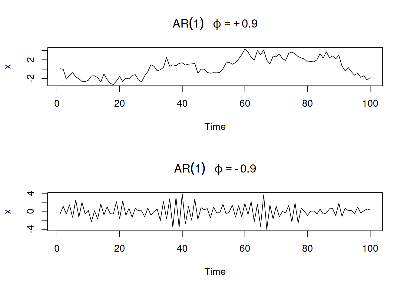
En este capítulo se introduce la familia de modelos ARIMA para series de tiempo. Se motiva su uso cuando la regresión clásica no captura toda la dinámica (p. ej., autocorrelación en residuos). Se presentan los modelos autorregresivos (AR), de media móvil (MA) y mixtos (ARMA), así como nociones de causalidad, invertibilidad y problemas de redundancia de parámetros. Se utilizan notación de operador de rezago y resultados sobre soluciones estacionarias, junto con ejemplos y código en R.
La regresión clásica es estática (solo entradas contemporáneas). En series de tiempo se desea permitir dependencia respecto a valores pasados de la propia serie y de entradas externas, lo cual abre la puerta a la predicción.
Modelo generador:
\[ x_t = x_{t-1} - 0.90\,x_{t-2} + w_t,\quad w_t \sim \text{WN}(0,\sigma_w^2=1). \]
Un pronóstico ingenuo:
\[ x_{n+1}^{\,n} = x_n - 0.90\,x_{n-1}. \]
Un modelo autorregresivo de orden \(p\) es
\[ \begin{equation*} x_t=\phi_1 x_{t-1}+\phi_2 x_{t-2}+\cdots+\phi_p x_{t-p}+w_t, \end{equation*} \]
donde \(x_t\) es estacionaria, \(w_t\sim wn(0,\sigma_w^2)\) y \(\phi_p\neq 0\). Si \(\mu=\mathrm{E}(x_t)\neq 0\), equivalentemente
\[ \begin{equation*} x_t=\alpha+\phi_1 x_{t-1}+\cdots+\phi_p x_{t-p}+w_t,\quad \alpha=\mu(1-\phi_1-\cdots-\phi_p). \end{equation*} \]
Con el operador \(B\), el modelo se escribe
\[ \begin{equation*} (1-\phi_1 B-\cdots-\phi_p B^p)\,x_t=w_t, \end{equation*} \]
o concisamente
\[ \begin{equation*} \phi(B)\,x_t=w_t, \end{equation*} \]
donde
\[ \begin{equation*} \phi(B)=1-\phi_1 B-\cdots-\phi_p B^p. \end{equation*} \]
Para \(x_t=\phi x_{t-1}+w_t\) e iterando hacia atrás:
\[ x_t=\phi^k x_{t-k}+\sum_{j=0}^{k-1}\phi^j w_{t-j}. \]
Si \(|\phi|<1\) y \(\sup_t \mathrm{var}(x_t)<\infty\), la solución estacionaria como proceso lineal es
\[ \begin{equation*} x_t=\sum_{j=0}^{\infty}\phi^j w_{t-j}. \end{equation*} \]
Con esto, \(\mathrm{E}(x_t)=0\) y la autocovarianza
\[ \begin{align*} \gamma(h) &=\mathrm{cov}(x_{t+h},x_t) =\sigma_w^2 \sum_{j=0}^{\infty}\phi^{h+j}\phi^j =\frac{\sigma_w^2\,\phi^{h}}{1-\phi^2},\quad h\ge 0. \end{align*} \]
Así, la ACF es
\[ \begin{equation*} \rho(h)=\frac{\gamma(h)}{\gamma(0)}=\phi^{h},\quad h\ge 0, \end{equation*} \]
y satisface
\[ \begin{equation*} \rho(h)=\phi\,\rho(h-1),\quad h=1,2,\ldots \end{equation*} \]
Comparación de \(\phi=0.9\) (trayectoria suave) vs \(\phi=-0.9\) (trayectoria “rugosa”):
par(mfrow=c(2,1))
plot(arima.sim(list(order=c(1,0,0), ar=.9), n=100), ylab="x",
main=(expression(AR(1)~~~phi==+.9)))
plot(arima.sim(list(order=c(1,0,0), ar=-.9), n=100), ylab="x",
main=(expression(AR(1)~~~phi==-.9)))
Para \(|\phi|>1\), se obtiene al iterar hacia adelante:
\[ \begin{align*} x_t&=\phi^{-k}x_{t+k}-\sum_{j=1}^{k-1}\phi^{-j}w_{t+j} \end{align*} \]
y, en el límite,
\[ \begin{equation*} x_t=-\sum_{j=1}^{\infty}\phi^{-j}w_{t+j}, \end{equation*} \]
que es estacionaria pero dependiente del futuro (no causal) y por tanto inútil para pronóstico.
Si \(x_t=\phi x_{t-1}+w_t\) con \(|\phi|>1\), existe un proceso causal equivalente
\[ y_t=\phi^{-1}y_{t-1}+v_t,\quad v_t\sim \text{iid }N\!\left(0,\sigma_w^2\phi^{-2}\right), \]
que es estocásticamente igual a \(x_t\) (misma familia finito-dimensional), ya que ambas comparten la misma estructura de covarianza:
\[\begin{aligned} \gamma_x(h) & =\operatorname{cov}\left(x_{t+h}, x_t\right)=\operatorname{cov}\left(-\sum_{j=1}^{\infty} \phi^{-j} w_{t+h+j},-\sum_{k=1}^{\infty} \phi^{-k} w_{t+k}\right) \\ & =\sigma_w^2 \phi^{-2} \phi^{-h} /\left(1-\phi^{-2}\right) \end{aligned}\]Si \(\phi(B)x_t=w_t\) y \(x_t=\psi(B)w_t=\sum_{j=0}^\infty \psi_j B^j w_t\), entonces
\[ \phi(B)\psi(B)w_t=w_t \;\Rightarrow\; (1-\phi B)\left(1+\psi_1 B+\psi_2 B^2+\cdots\right)=1. \]
Igualando coeficientes se obtiene \(\psi_j=\phi^j\). En general, tratar \(B\) como \(z\) complejo:
\[ \phi^{-1}(z)=\frac{1}{1-\phi z}=\sum_{j=0}^{\infty}\phi^j z^j,\quad |z|\le 1. \]
\[ \begin{equation*} x_t=w_t+\theta_1 w_{t-1}+\cdots+\theta_q w_{t-q}, \end{equation*} \]
con \(w_t\sim wn(0,\sigma_w^2)\) y \(\theta_q\neq 0\). Equivalentemente,
\[ \begin{equation*} x_t=\theta(B)w_t, \end{equation*} \]
donde el operador MA es
\[ \begin{equation*} \theta(B)=1+\theta_1 B+\cdots+\theta_q B^q. \end{equation*} \]
Los procesos MA son estacionarios para cualquier \((\theta_1,\ldots,\theta_q)\).
Para \(x_t=w_t+\theta w_{t-1}\), \(\mathrm{E}(x_t)=0\) y
\[ \gamma(h)= \begin{cases} (1+\theta^2)\sigma_w^2, & h=0,\\ \theta\,\sigma_w^2, & h=1,\\ 0, & h>1, \end{cases} \quad \rho(h)= \begin{cases} \dfrac{\theta}{1+\theta^2}, & h=1,\\ 0, & h>1. \end{cases} \]
par(mfrow = c(2,1))
plot(arima.sim(list(order=c(0,0,1), ma=.9), n=100), ylab="x",
     main=(expression(MA(1)~~~theta==+.5)))
plot(arima.sim(list(order=c(0,0,1), ma=-.9), n=100), ylab="x",
     main=(expression(MA(1)~~~theta==-.5)))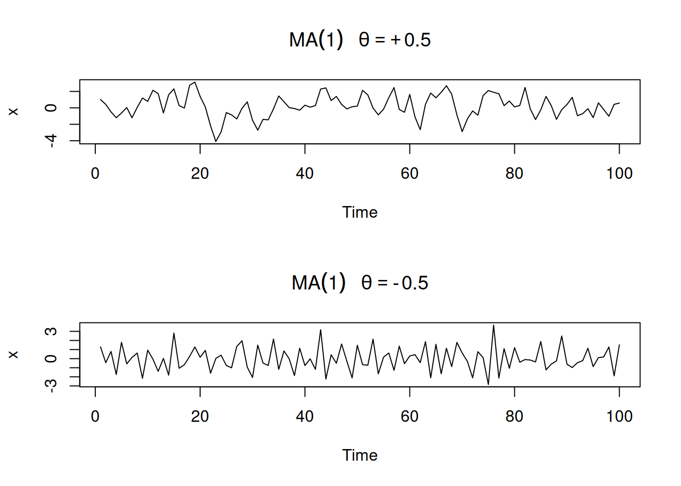
Para MA(1), \(\rho(h)\) es igual para \(\theta\) y \(1/\theta\); distintos pares \((\sigma_w^2,\theta)\) pueden inducir la misma \(\gamma(h)\): por ejemplo tomando \(\theta=5\) y \(\sigma^2_w=1\) o \(\theta=1/5\) y \(\sigma^2_w=25\). Se elige la representación invertible: aquella con \(|\theta|<1\), que permite
\[ w_t=\sum_{j=0}^{\infty}(-\theta)^j x_{t-j}. \]
Vía operadores: si \(\theta(B)=1+\theta B\), entonces para \(|\theta|<1\),
\[ \pi(B)=\theta^{-1}(B)=\sum_{j=0}^{\infty}(-\theta)^j B^j. \]
Una serie \({x_t}\) es ARMA\((p,q)\) si es estacionaria y
\[ \begin{equation*} x_t=\phi_1 x_{t-1}+\cdots+\phi_p x_{t-p}+w_t+\theta_1 w_{t-1}+\cdots+\theta_q w_{t-q}, \end{equation*} \]
con \(\phi_p\neq 0\), \(\theta_q\neq 0\), \(\sigma_w^2>0\). Si \(\mu\neq 0\),
\[ \begin{equation*} x_t=\alpha+\phi_1 x_{t-1}+\cdots+\phi_p x_{t-p}+w_t+\theta_1 w_{t-1}+\cdots+\theta_q w_{t-q}, \end{equation*} \]
y, en forma concisa,
\[ \begin{equation*} \phi(B)\,x_t=\theta(B)\,w_t. \end{equation*} \]
Partiendo de \(x_t=w_t\) y multiplicando por \(\eta(B)=1-0.5B\):
\[ \begin{equation*} x_t=0.5\,x_{t-1}-0.5\,w_{t-1}+w_t, \end{equation*} \]
que parece un ARMA(1,1) pero es ruido blanco: hay sobre–parametrización.
Demostración empírica de sobre–parametrización al ajustar ARMA(1,1) a datos iid:
set.seed(8675309)
x = rnorm(150, mean=5) # iid N(5,1)
arima(x, order=c(1,0,1)) # estimación
Call:
arima(x = x, order = c(1, 0, 1))

Coefficients:
          ar1     ma1  intercept
      -0.9595  0.9527     5.0462
s.e.   0.1688  0.1750     0.0727

sigma^2 estimated as 0.7986:  log likelihood = -195.98,  aic = 399.96
# Coeficientes típicos: ar1 ~ -0.96, ma1 ~ 0.95, ambos "significativos"\[ \begin{equation*} \phi(z)=1-\phi_1 z-\cdots-\phi_p z^p,\quad \phi_p\neq 0; \end{equation*} \]
\[ \begin{equation*} \theta(z)=1+\theta_1 z+\cdots+\theta_q z^q,\quad \theta_q\neq 0. \end{equation*} \]
Forma mínima: \(\phi(z)\) y \(\theta(z)\) sin factores comunes (evita redundancia).
ARMA\((p,q)\) es causal si puede escribirse como proceso lineal unilateral
\[ \begin{equation*} x_t=\sum_{j=0}^{\infty}\psi_j w_{t-j}=\psi(B)w_t,\quad \sum_{j=0}^{\infty}|\psi_j|<\infty,\ \psi_0=1. \end{equation*} \]
ARMA\((p,q)\) es causal si y solo si \(\phi(z)\neq 0\) para \(|z|\le 1\). Los pesos \(\psi_j\) satisfacen
\[ \psi(z)=\sum_{j=0}^{\infty}\psi_j z^j=\frac{\theta(z)}{\phi(z)},\quad |z|\le 1. \]
ARMA\((p,q)\) es invertible si existe
\[ \begin{equation*} \pi(B)x_t=\sum_{j=0}^{\infty}\pi_j x_{t-j}=w_t,\quad \sum_{j=0}^{\infty}|\pi_j|<\infty,\ \pi_0=1. \end{equation*} \]
ARMA\((p,q)\) es invertible si y solo si \(\theta(z)\neq 0\) para \(|z|\le 1\), y
\[ \pi(z)=\sum_{j=0}^{\infty}\pi_j z^j=\frac{\phi(z)}{\theta(z)},\quad |z|\le 1. \]
Dado
\[ x_t=0.4\,x_{t-1}+0.45\,x_{t-2}+w_t+w_{t-1}+0.25\,w_{t-2}, \]
u operador:
\[ (1-0.4B-0.45B^2)\,x_t=(1+B+0.25B^2)\,w_t. \]
Factorizando:
\[ \phi(B)=(1+0.5B)(1-0.9B),\quad \theta(B)=(1+0.5B)^2. \]
Cancelando el factor común \((1+0.5B)\):
\[ \begin{equation*} (1-0.9B)\,x_t=(1+0.5B)\,w_t \;\Rightarrow\; x_t=0.9\,x_{t-1}+0.5\,w_{t-1}+w_t, \end{equation*} \]
que es ARMA(1,1), causal (raíz de \(\phi(z)=1-0.9z\) es \(z=10/9>1\)) e invertible (raíz de \(\theta(z)=1+0.5z\) es \(z=-2\)).
Pesos \(\psi_j\) (linealización vía \(\phi(z)\psi(z)=\theta(z)\)):
\[ (1-0.9 z)\left(1+\psi_1 z+\psi_2 z^2+\cdots\right)=1+0.5 z \;\Rightarrow\; \psi_1=1.4,\ \psi_j=0.9\,\psi_{j-1}\ (j>1), \]
de modo que \(\psi_j=1.4(0.9)^{j-1},, j\ge 1\) y
\[ x_t=w_t+1.4\sum_{j=1}^{\infty} 0.9^{\,j-1} w_{t-j}. \]
En R:
ARMAtoMA(ar=.9, ma=.5, 10) # primeros 10 psi-weights [1] 1.4000000 1.2600000 1.1340000 1.0206000 0.9185400 0.8266860 0.7440174
[8] 0.6696157 0.6026541 0.5423887Pesos \(\pi_j\) (invertibilidad vía \(\theta(z)\pi(z)=\phi(z)\)):
\[ (1+0.5z)\left(1+\pi_1 z+\pi_2 z^2+\cdots\right)=1-0.9z \;\Rightarrow\; \pi_j=(-1)^j\,1.4\,(0.5)^{\,j-1},\ j\ge 1, \]
y como \(w_t=\sum_{j=0}^{\infty}\pi_j x_{t-j}\),
\[ x_t=1.4\sum_{j=1}^{\infty}(-0.5)^{\,j-1} x_{t-j}+w_t. \]
ARMAtoMA(ar=-.5, ma=-.9, 10) # primeros 10 pi-weights [1] -1.400000000 0.700000000 -0.350000000 0.175000000 -0.087500000
[6] 0.043750000 -0.021875000 0.010937500 -0.005468750 0.002734375Para \((1-\phi_1 B-\phi_2 B^2)\,x_t=w_t\) es causal si las raíces de \(\phi(z)=1-\phi_1 z-\phi_2 z^2\) están fuera del círculo unidad. Equivalente en parámetros: \[ \begin{equation*} \phi_1+\phi_2<1,\quad \phi_2-\phi_1<1,\quad |\phi_2|<1. \end{equation*} \] (Define una región triangular de causalidad en el plano \((\phi_1,\phi_2)\).)
# (Opcional) Visualización de la región causal AR(2) con ggplot2:
# Grid de parámetros y prueba de desigualdades
grid <- expand_grid(phi1 = seq(-2, 2, by = 0.01),
                    phi2 = seq(-1, 1, by = 0.01)) |>
  mutate(causal = (phi1 + phi2 < 1) & (phi2 - phi1 < 1) & (abs(phi2) < 1))

ggplot(grid, aes(phi1, phi2, fill = causal)) +
  geom_raster() +
  scale_fill_manual(values = c("TRUE"="#4daf4a","FALSE"="#f0f0f0")) +
  labs(x=expression(phi[1]), y=expression(phi[2]),
       title="Región de causalidad para AR(2)") +
  theme_minimal()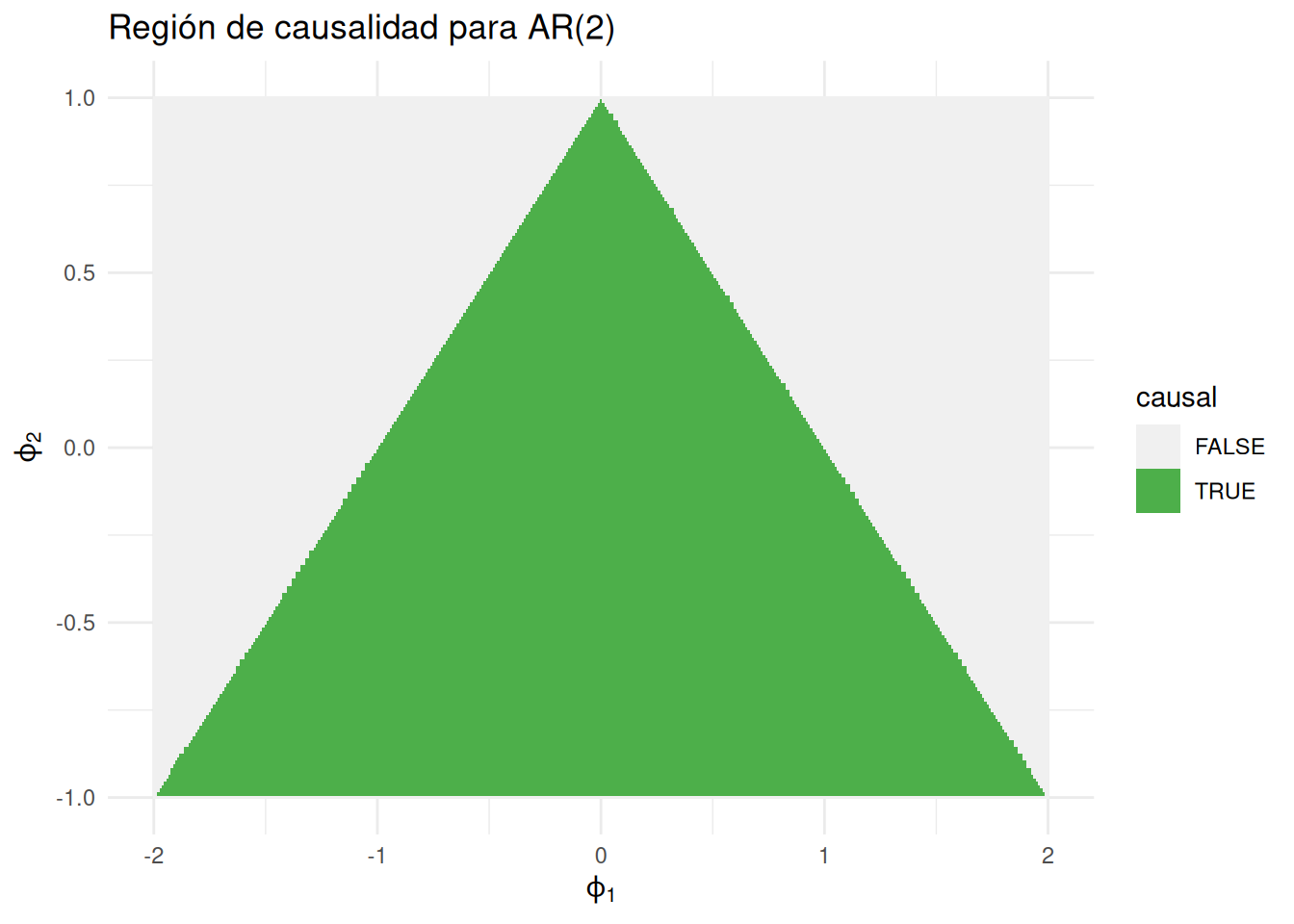
En esta sección se estudian las ecuaciones en diferencias y su relación con los procesos ARMA y sus funciones de autocorrelación. Se presentan las soluciones para ecuaciones homogéneas de primer y segundo orden, su generalización al caso de orden \(p\), y se muestran aplicaciones al cálculo de funciones de autocorrelación y de los pesos \(\psi\) en modelos ARMA.
Consideremos la secuencia \(u_{0}, u_{1}, u_{2}, \ldots\) que satisface:
\[ u_{n} - \alpha u_{n-1} = 0, \quad \alpha \neq 0, \quad n=1,2,\ldots \]
Ejemplo: la ACF de un AR(1) cumple:
\[ \rho(h) - \phi \rho(h-1) = 0, \quad h=1,2,\ldots \]
La solución es:
\[ u_{n} = \alpha^n u_0 \]
con condición inicial \(u_{0}=c\), se tiene \(u_{n} = \alpha^n c\).
En notación operador:
\[ (1 - \alpha B)u_n = 0 \]
y el polinomio asociado es \(\alpha(z) = 1 - \alpha z\), con raíz \(z_0 = 1/\alpha\). La solución:
\[ u_{n} = \alpha^n c = (z_0^{-1})^n c \]
Ahora supongamos:
\[ u_n - \alpha_1 u_{n-1} - \alpha_2 u_{n-2} = 0, \quad \alpha_2 \neq 0, \quad n=2,3,\ldots \]
El polinomio asociado es:
\[ \alpha(z) = 1 - \alpha_1 z - \alpha_2 z^2 \]
con raíces \(z_1, z_2\).
\[ u_n = c_1 z_1^{-n} + c_2 z_2^{-n} \]
\[ u_n = z_0^{-n}(c_1 + c_2 n) \]
La ecuación en diferencias:
\[ u_n - \alpha_1 u_{n-1} - \cdots - \alpha_p u_{n-p} = 0, \quad \alpha_p \neq 0 \]
con polinomio asociado \(\alpha(z) = 1 - \alpha_1 z - \cdots - \alpha_p z^p\).
La solución general es:
\[ u_n = z_1^{-n} P_1(n) + z_2^{-n} P_2(n) + \cdots + z_r^{-n} P_r(n) \]
donde \(z_j\) son raíces con multiplicidad \(m_j\) y \(P_j(n)\) son polinomios de grado \(m_j - 1\).
Sea:
\[ x_t = \phi_1 x_{t-1} + \phi_2 x_{t-2} + w_t \]
Se obtiene:
\[ \gamma(h) = \phi_1 \gamma(h-1) + \phi_2 \gamma(h-2), \quad h=1,2,\ldots \]
Dividiendo por \(\gamma(0)\):
\[ \rho(h) - \phi_1 \rho(h-1) - \phi_2 \rho(h-2) = 0, \quad h=1,2,\ldots \]
La solución depende de las raíces de \(\phi(z) = 1 - \phi_1 z - \phi_2 z^2\):
Raíces reales distintas: \(\rho(h) = c_1 z_1^{-h} + c_2 z_2^{-h}\)
Raíz doble: \(\rho(h) = z_0^{-h}(c_1 + c_2 h)\)
Raíces complejas conjugadas: \(\rho(h) = a |z_1|^{-h} \cos(h\theta + b)\)
Supongamos que las raíces son \(z_{1}\) y \(z_{2} = \bar{z}_{1}\), es decir, un par conjugado complejo. En este caso, los coeficientes de la solución cumplen \(c_{2} = \bar{c}_{1}\), ya que la función de autocorrelación \(\rho(h)\) debe ser un número real.
La solución general para \(\rho(h)\) es:
\[ \rho(h) = c_{1} z_{1}^{-h} + \bar{c}_{1} \bar{z}_{1}^{-h}. \]
Recordemos que cualquier número complejo \(z = x + iy\) se puede escribir en forma polar como:
\[ z = |z|(\cos \theta + i \sin \theta), \]
donde:
De forma compacta, esta representación se escribe como:
\[ z = |z| e^{i\theta}. \]
Aplicando esto a \(z_{1}\):
\[ z_{1} = |z_{1}| e^{i\theta}. \]
De aquí se sigue que:
\[ z_{1}^{-h} = |z_{1}|^{-h} e^{-i h \theta}. \]
Como \(c_{1}\) también puede escribirse en forma polar, la expresión completa de \(\rho(h)\) se puede reorganizar usando la identidad de Euler:
\[ e^{i\alpha} + e^{-i\alpha} = 2\cos(\alpha). \]
De este modo, la solución toma la forma:
\[ \rho(h) = a |z_{1}|^{-h} \cos(h\theta + b), \]
donde:
Modelo:
\[ x_t = 1.5 x_{t-1} - 0.75 x_{t-2} + w_t \]
Polinomio: \(\phi(z) = 1 - 1.5z + 0.75z^2\).
Las raíces: \(1 \pm i/\sqrt{3}\), con \(\theta = \tan^{-1}(1/\sqrt{3}) = 2\pi/12\).
En R:
z <- c(1,-1.5,.75)
a <- polyroot(z)[1]
a
[1] 1+0.5773503iarg <- Arg(a)/(2*pi)
1/arg[1] 12Simulación:
set.seed(8675309)
ar2 <- arima.sim(list(order=c(2,0,0), ar=c(1.5,-.75)), n=144)
ar2 %>%
  tsibble::as_tsibble() %>%
  ggplot(aes(index, value)) +
  geom_line() +
  labs(x="Tiempo", y="Serie simulada")
Registered S3 method overwritten by 'tsibble':
method from
as_tibble.grouped_df dplyr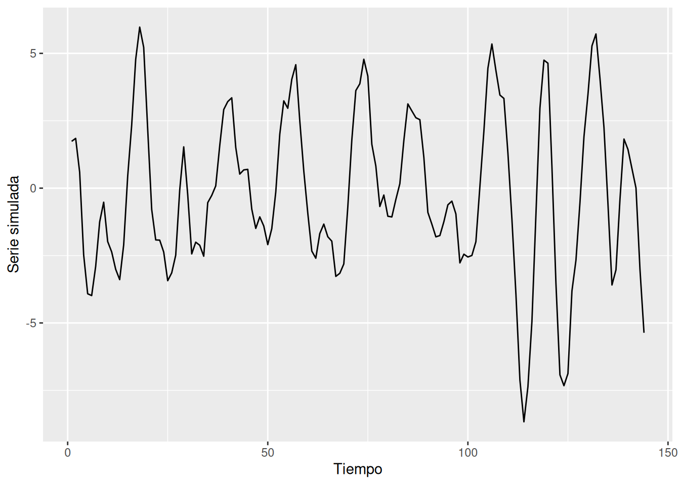
ACF en R:
acf_vals <- ARMAacf(ar=c(1.5,-.75), ma=0, lag.max=50)
tibble(lag=0:50, acf=acf_vals) %>%
  ggplot(aes(lag, acf)) +
  geom_col() +
  geom_hline(yintercept=0, color="red")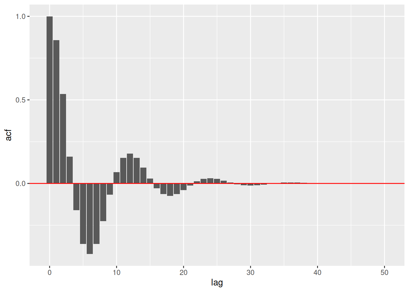
Para un ARMA(\(p,q\)):
\[ \phi(B)x_t = \theta(B)w_t \]
con expansión:
\[ x_t = \sum_{j=0}^\infty \psi_j w_{t-j} \]
Las condiciones son:
\[ \psi_j - \sum_{k=1}^p \phi_k \psi_{j-k} = 0, \quad j \geq \max(p,q+1) \]
y
\[ \psi_j - \sum_{k=1}^j \phi_k \psi_{j-k} = \theta_j, \quad 0 \leq j < \max(p,q+1) \]
Ejemplo:
\[ x_t = 0.9 x_{t-1} + 0.5 w_{t-1} + w_t \]
Se obtiene \(\psi_0 = 1\), \(\psi_1 = 1.4\), y en general:
\[ \psi_j = 1.4 (0.9)^{j-1}, \quad j \geq 1 \]
En R:
ARMAtoMA(ar=0.9, ma=0.5, 50) %>%
  tibble(lag=1:50, psi=.) %>%
  ggplot(aes(lag, psi)) +
  geom_line() +
  labs(x="Rezago", y="Peso psi")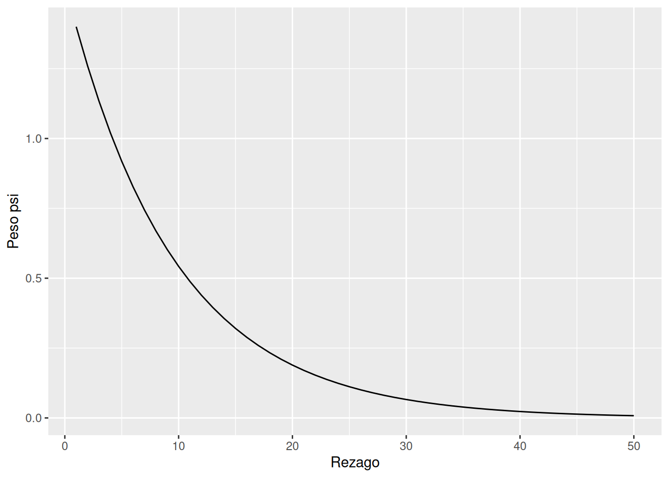
En esta sección se estudian las funciones de autocorrelación (ACF) y autocorrelación parcial (PACF) para procesos de series de tiempo. Se muestran sus propiedades en modelos MA, AR y ARMA, así como su utilidad para la identificación del orden de dependencia en estos procesos. Además, se presentan ejemplos numéricos y código en R para ilustrar los cálculos.
Un proceso \(x_t = \theta(B) w_t\), con \(\theta(B) = 1 + \theta_1 B + \cdots + \theta_q B^q\), tiene media cero y función de autocovarianza:
\[ \gamma(h) = \begin{cases} \sigma_w^2 \sum_{j=0}^{q-h} \theta_j \theta_{j+h}, & 0 \leq h \leq q \\ 0, & h > q \end{cases} \]
Al dividir por \(\gamma(0)\), se obtiene la ACF:
\[ \rho(h) = \begin{cases} \dfrac{\sum_{j=0}^{q-h} \theta_j \theta_{j+h}}{1+\theta_1^2+\cdots+\theta_q^2}, & 1 \leq h \leq q \\ 0, & h > q \end{cases} \]
Para un ARMA causal \(\phi(B) x_t = \theta(B) w_t\), se escribe:
\[ x_t = \sum_{j=0}^\infty \psi_j w_{t-j} \]
con \(\mathrm{E}(x_t)=0\) y
\[ \gamma(h) = \sigma_w^2 \sum_{j=0}^\infty \psi_j \psi_{j+h}, \quad h \geq 0 \]
La ecuación de recurrencia para \(\gamma(h)\) es:
\[ \gamma(h) - \phi_1 \gamma(h-1) - \cdots - \phi_p \gamma(h-p) = 0, \quad h \geq \max(p, q+1) \]
con condiciones iniciales:
\[ \gamma(h) - \sum_{j=1}^p \phi_j \gamma(h-j) = \sigma_w^2 \sum_{j=h}^q \theta_j \psi_{j-h}, \quad 0 \leq h < \max(p,q+1) \]
Se cumple:
\[ \rho(h) - \phi_1 \rho(h-1) - \cdots - \phi_p \rho(h-p) = 0, \quad h \geq p \]
La solución general es:
\[ \rho(h) = z_1^{-h} P_1(h) + \cdots + z_r^{-h} P_r(h), \quad h \geq p \]
donde \(z_i\) son raíces de \(\phi(z)\) y \(P_j(h)\) son polinomios.
Considere el proceso ARMA(1,1) \(x_{t}=\phi\, x_{t-1}+\theta\, w_{t-1}+w_{t}\), donde \(|\phi|<1\). La función de autocovarianza satisface
\[ \gamma(h)-\phi\, \gamma(h-1)=0, \quad h=2,3,\ldots \]
y por lo tanto la solución general es
\[ \begin{equation*} \gamma(h)=c\, \phi^{h}, \quad h=1,2,\ldots \end{equation*} \]
Para obtener las condiciones iniciales usamos:
\[ \gamma(0)=\phi\, \gamma(1)+\sigma_{w}^{2}\big[1+\theta \phi+\theta^{2}\big] \quad \text{y} \quad \gamma(1)=\phi\, \gamma(0)+\sigma_{w}^{2}\theta . \]
Al resolver para \(\gamma(0)\) y \(\gamma(1)\), obtenemos:
\[ \gamma(0)=\sigma_{w}^{2}\,\frac{1+2\theta \phi+\theta^{2}}{1-\phi^{2}} \quad \text{y} \quad \gamma(1)=\sigma_{w}^{2}\,\frac{(1+\theta \phi)(\phi+\theta)}{1-\phi^{2}} . \]
Para resolver \(c\), note que, \(\gamma(1)=c\,\phi\), es decir, \(c=\gamma(1)/\phi\). Por lo tanto, la solución específica para \(h \ge 1\) es
\[ \gamma(h)=\frac{\gamma(1)}{\phi}\,\phi^{h} =\sigma_{w}^{2}\,\frac{(1+\theta \phi)(\phi+\theta)}{1-\phi^{2}}\,\phi^{\,h-1}. \]
Finalmente, al dividir por \(\gamma(0)\) se obtiene la ACF
\[ \begin{equation*} \rho(h)=\frac{(1+\theta \phi)(\phi+\theta)}{1+2\theta \phi+\theta^{2}}\,\phi^{\,h-1}, \quad h \ge 1 \end{equation*} \]
Obsérvese que el patrón general de \(\rho(h)\) frente a \(h\) no es distinto del de un AR(1). Por lo tanto, es poco probable que podamos distinguir entre un \(\operatorname{ARMA}(1,1)\) y un \(\operatorname{AR}(1)\) basándonos únicamente en una ACF estimada a partir de una muestra. Esta consideración nos llevará a la función de autocorrelación parcial.
Anteriormente vimos que, para un modelo MA(\(q\)), la función de autocorrelación (ACF) se anula para rezagos mayores que \(q\). Además, como \(\theta_q \neq 0\), la ACF no es cero en el rezago \(q\). Esto significa que la ACF aporta bastante información sobre el orden de dependencia en procesos de media móvil.
Sin embargo, si el proceso es ARMA o AR, la ACF por sí sola no permite identificar claramente el orden. Por ello, se introduce la función de autocorrelación parcial (PACF), que se comporta para los modelos AR de forma similar a la ACF en los modelos MA.
Si \(X\), \(Y\) y \(Z\) son variables aleatorias, la correlación parcial entre \(X\) y \(Y\) dado \(Z\) se obtiene mediante:
\[ \rho_{XY|Z} = \operatorname{corr}\{X - \hat{X}, \, Y - \hat{Y}\}. \]
La idea es medir la asociación de \(X\) y \(Y\) una vez eliminada la influencia lineal de \(Z\). En el caso normal multivariado, esta definición coincide con:
\[ \rho_{XY|Z} = \operatorname{corr}(X,Y \mid Z). \]
Consideremos un modelo causal AR(1):
\[ x_t = \phi x_{t-1} + w_t. \]
El cálculo de la covarianza en el rezago 2 es:
\[ \begin{aligned} \gamma_x(2) &= \operatorname{cov}(x_t, x_{t-2}) \\ &= \operatorname{cov}(\phi x_{t-1} + w_t, \, x_{t-2}) \\ &= \operatorname{cov}(\phi^2 x_{t-2} + \phi w_{t-1} + w_t, \, x_{t-2}) \\ &= \phi^2 \gamma_x(0). \end{aligned} \]
Este resultado se debe a la causalidad: \(x_{t-2}\) depende de \({w_{t-2}, w_{t-3},\ldots}\), que son no correlacionados con \(w_t\) y \(w_{t-1}\). Así, \(x_t\) y \(x_{t-2}\) están correlacionados a través de \(x_{t-1}\).
Para romper esta cadena de dependencia, eliminamos el efecto de \(x_{t-1}\):
\[ \operatorname{cov}\big(x_t - \phi x_{t-1}, \, x_{t-2} - \phi x_{t-1}\big) = \operatorname{cov}(w_t, x_{t-2} - \phi x_{t-1}) = 0. \]
De aquí surge la PACF: la correlación entre \(x_s\) y \(x_t\) una vez eliminada la influencia de las variables intermedias.
Para una serie estacionaria de media cero:
\[ \hat{x}_{t+h} = \beta_1 x_{t+h-1} + \beta_2 x_{t+h-2} + \cdots + \beta_{h-1} x_{t+1}. \]
\[ \hat{x}_t = \beta_1 x_{t+1} + \beta_2 x_{t+2} + \cdots + \beta_{h-1} x_{t+h-1}. \]
Por estacionariedad, los coeficientes \(\beta_1, \ldots, \beta_{h-1}\) son iguales en ambas expresiones.
Formalmente, la PACF mide la correlación entre \(x_{t+h}\) y \(x_t\) eliminando el efecto lineal de los valores intermedios. Formalmente:
\[ \phi_{hh} = \operatorname{corr}(x_{t+h} - \hat{x}_{t+h}, x_t - \hat{x}_t) \]
donde \(\hat{x}_{t+h}\) y \(\hat{x}_t\) son regresiones sobre los valores intermedios.
Consideremos el proceso AR(1):
\[ x_t = \phi x_{t-1} + w_t, \quad |\phi| < 1. \]
Por definición, el primer valor de la PACF es simplemente:
\[ \phi_{11} = \rho(1) = \phi. \]
Cálculo de \(\phi_{22}\)
Regresión de \(x_{t+2}\) sobre \(x_{t+1}\) Supongamos \(\hat{x}_{t+2} = \beta x_{t+1}\). Para encontrar \(\beta\), minimizamos el error cuadrático esperado:
\[ \mathrm{E}\left[(x_{t+2} - \hat{x}_{t+2})^2\right] = \mathrm{E}\left[(x_{t+2} - \beta x_{t+1})^2\right] = \gamma(0) - 2\beta \gamma(1) + \beta^2 \gamma(0). \]
Derivando respecto a \(\beta\) y resolviendo, se obtiene:
\[ \beta = \frac{\gamma(1)}{\gamma(0)} = \rho(1) = \phi. \]
Regresión de \(x_t\) sobre \(x_{t+1}\) Supongamos \(\hat{x}_t = \beta x_{t+1}\). Nuevamente, al minimizar:
\[ \mathrm{E}\left[(x_t - \hat{x}_t)^2\right] = \mathrm{E}\left[(x_t - \beta x_{t+1})^2\right] = \gamma(0) - 2\beta \gamma(1) + \beta^2 \gamma(0), \] Con estos valores:
\[ \begin{aligned} \phi_{22} &= \operatorname{corr}(x_{t+2} - \hat{x}_{t+2}, \, x_t - \hat{x}_t) \\ &= \operatorname{corr}(x_{t+2} - \phi x_{t+1}, \, x_t - \phi x_{t+1}) \\ &= \operatorname{corr}(w_{t+2}, \, x_t - \phi x_{t+1}) \\ &= 0, \end{aligned} \]
debido a la causalidad: \(w_{t+2}\) es no correlacionado con las variables del pasado.
Para \(h > p\), \(\phi_{hh} = 0\) por causalidad. La PACF corta en el rezago \(p\).
Código en R:
ACF <- ARMAacf(ar=c(1.5, -0.75), ma=0, 24)[-1]
PACF <- ARMAacf(ar=c(1.5, -0.75), ma=0, 24, pacf=TRUE)

par(mfrow=c(1,2))
plot(ACF, type="h", xlab="Rezago", ylim=c(-0.8,1)); abline(h=0)
plot(PACF, type="h", xlab="Rezago", ylim=c(-0.8,1)); abline(h=0)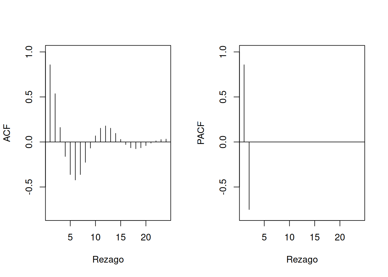
Para un MA(1), \(x_t = w_t + \theta w_{t-1}\):
\[ \phi_{hh} = -\frac{(-\theta)^h (1-\theta^2)}{1-\theta^{2(h+1)}}, \quad h \geq 1 \]
En general, la PACF de un MA no corta, a diferencia de un AR.
Con 453 meses de datos (1950–1987), la ACF muestra ciclos de 12 meses y la PACF valores altos en \(h=1,2\), sugiriendo un AR(2):
\[ x_t = \phi_0 + \phi_1 x_{t-1} + \phi_2 x_{t-2} + w_t \]
Estimaciones:
Código en R:
acf2(rec, 48) # ACF y PACF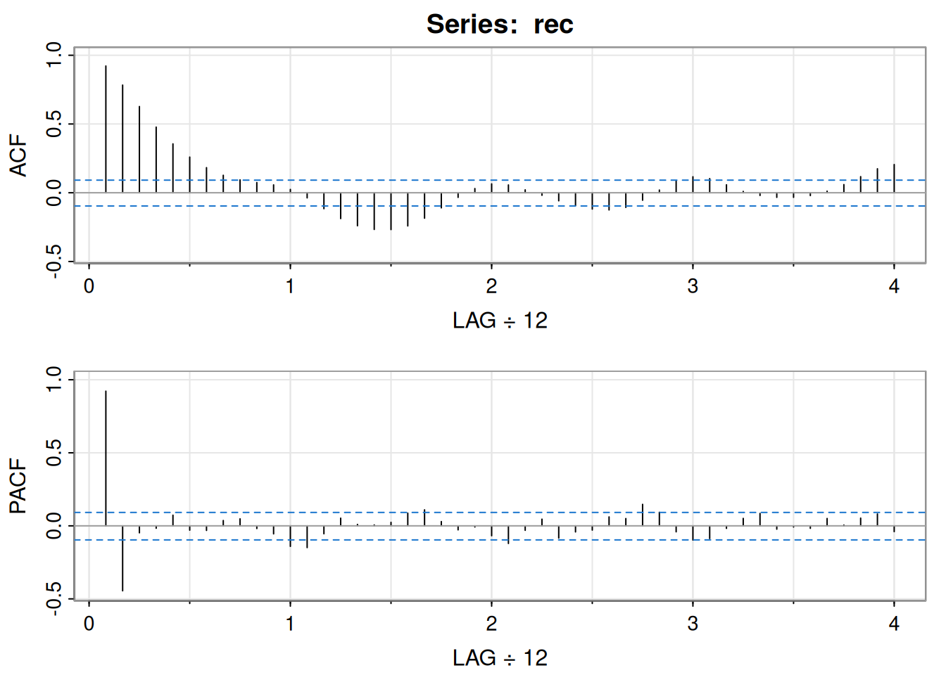
     [,1]  [,2]  [,3]  [,4] [,5]  [,6]  [,7] [,8] [,9] [,10] [,11] [,12] [,13]
ACF  0.92  0.78  0.63  0.48 0.36  0.26  0.18 0.13 0.09  0.07  0.06  0.02 -0.04
PACF 0.92 -0.44 -0.05 -0.02 0.07 -0.03 -0.03 0.04 0.05 -0.02 -0.05 -0.14 -0.15
     [,14] [,15] [,16] [,17] [,18] [,19] [,20] [,21] [,22] [,23] [,24] [,25]
ACF  -0.12 -0.19 -0.24 -0.27 -0.27 -0.24 -0.19 -0.11 -0.03  0.03  0.06  0.06
PACF -0.05  0.05  0.01  0.01  0.02  0.09  0.11  0.03 -0.03 -0.01 -0.07 -0.12
     [,26] [,27] [,28] [,29] [,30] [,31] [,32] [,33] [,34] [,35] [,36] [,37]
ACF   0.02 -0.02 -0.06 -0.09 -0.12 -0.13 -0.11 -0.05  0.02  0.08  0.12  0.10
PACF -0.03  0.05 -0.08 -0.04 -0.03  0.06  0.05  0.15  0.09 -0.04 -0.10 -0.09
     [,38] [,39] [,40] [,41] [,42] [,43] [,44] [,45] [,46] [,47] [,48]
ACF   0.06  0.01 -0.02 -0.03 -0.03 -0.02  0.01  0.06  0.12  0.17  0.20
PACF -0.02  0.05  0.08 -0.02 -0.01 -0.02  0.05  0.01  0.05  0.08 -0.04
regr <- ar.ols(rec, order=2, demean=FALSE, intercept=TRUE)
regr$asy.se.coef # errores estándar$x.mean
[1] 1.110599
$ar
[1] 0.04178901 0.04187942| Modelo | ACF | PACF |
|---|---|---|
| AR(p) | Decae | Corta en p |
| MA(q) | Corta en q | Decae |
| ARMA(p,q) | Decae | Decae |
Este apartado presenta los fundamentos del pronóstico en series de tiempo estacionarias con parámetros conocidos. Se define el mejor predictor en media cuadrática como una esperanza condicional y, dentro de los predictores lineales, se desarrollan los mejores predictores lineales (BLP). Se introducen ecuaciones de predicción en forma escalar y matricial, el algoritmo de Durbin–Levinson, el algoritmo de innovaciones, así como la formulación de pronósticos ARMA (incluyendo versiones truncadas), pronósticos de largo plazo y backcasting.
Dado \(x_{1:n}={x_1,\dots,x_n}\) y una serie estacionaria \(x_t\) con parámetros conocidos, el objetivo es predecir \(x_{n+m}\), \(m=1,2,\ldots\). El predictor que minimiza el error cuadrático medio (MMCE) es
\[ x_{n+m}^{\,n}=\mathrm{E}\!\left(x_{n+m}\mid x_{1:n}\right), \]
pues minimiza
\[ \mathrm{E}\!\left[x_{n+m}-g(x_{1:n})\right]^2. \]
Se restringe la atención a predictores lineales:
\[ x_{n+m}^{\,n}=\alpha_0+\sum_{k=1}^n \alpha_k x_k, \]
donde los coeficientes dependen de \(n\) y \(m\). Los BLP son aquellos que minimizan (en el conjunto lineal) el error cuadrático. Bajo gaussianidad, MMCE y BLP coinciden.
Propiedad (Mejor predicción lineal para procesos estacionarios). Dado \(x_{1},\ldots,x_n\), el BLP \(x_{n+m}^{,n}=\alpha_0+\sum_{k=1}^n \alpha_k x_k\) satisface
\[ \mathrm{E}\!\left[\left(x_{n+m}-x_{n+m}^{\,n}\right)x_k\right]=0,\quad k=0,1,\ldots,n, \]
donde \(x_0=1\), para resolver \({\alpha_0,\alpha_1,\ldots,\alpha_n}\). Si \(\mathrm{E}(x_t)=\mu\), el primer momento implica \(\mathrm{E}(x_{n+m}^{,n})=\mu\) y
\[ \alpha_0=\mu\Big(1-\sum_{k=1}^n \alpha_k\Big), \]
por lo que, sin pérdida de generalidad (mientras no estimemos), se toma \(\mu=0\) y \(\alpha_0=0\).
El BLP un paso adelante tiene forma
\[ x_{n+1}^{\,n}=\phi_{n1}x_n+\phi_{n2}x_{n-1}+\cdots+\phi_{nn}x_1. \]
Los coeficientes satisfacen
\[ \sum_{j=1}^n \phi_{nj}\,\gamma(k-j)=\gamma(k),\quad k=1,\ldots,n, \]
que en notación matricial son
\[ \Gamma_n\,\phi_n=\gamma_n, \]
con \(\Gamma_n={\gamma(k-j)}_{j,k=1}^n\), \(\phi_n=(\phi_{n1},\ldots,\phi_{nn})'\) y \(\gamma_n=(\gamma(1),\ldots,\gamma(n))'\). Si \(\Gamma_n\) es no singular,
\[ \phi_n=\Gamma_n^{-1}\gamma_n. \]
El error cuadrático medio (ECM) un paso adelante es
\[ P_{n+1}^{\,n}=\mathrm{E}\!\left(x_{n+1}-x_{n+1}^{\,n}\right)^2=\gamma(0)-\gamma_n'\Gamma_n^{-1}\gamma_n. \]
Para \(x_t=\phi_1x_{t-1}+\phi_2x_{t-2}+w_t\) causal:
\[ x_2^{\,1}=\phi_{11}x_1=\frac{\gamma(1)}{\gamma(0)}x_1=\rho(1)x_1. \]
\[ x_3^{\,2}=\phi_{21}x_2+\phi_{22}x_1, \]
y por el modelo, \(x_3^{,2}=\phi_1x_2+\phi_2x_1\), de modo que \(\phi_{21}=\phi_1,\ \phi_{22}=\phi_2\). En general, para \(n\ge2\):
\[ x_{n+1}^{\,n}=\phi_1x_n+\phi_2x_{n-1}. \]
Generalización AR(\(p\)): para \(n\ge p\),
\[ x_{n+1}^{\,n}=\phi_1x_n+\phi_2x_{n-1}+\cdots+\phi_p x_{n-p+1}. \]
El sistema \(\Gamma_n \phi_n = \gamma_n\) es costoso de resolver para grandes \(n\). Para evitar invertir matrices grandes, se usan soluciones recursivas:
\[ \phi_{00}=0,\quad P_{1}^{\,0}=\gamma(0). \]
\[ \phi_{nn}=\frac{\rho(n)-\sum_{k=1}^{n-1}\phi_{n-1,k}\rho(n-k)}{1-\sum_{k=1}^{n-1}\phi_{n-1,k}\rho(k)},\qquad P_{n+1}^{\,n}=P_n^{\,n-1}\left(1-\phi_{nn}^2\right), \]
y, para \(k=1,\ldots,n-1\),
\[ \phi_{nk}=\phi_{n-1,k}-\phi_{nn}\,\phi_{n-1,n-k}. \]
Error de predicción un paso adelante (forma producto):
\[ P_{n+1}^{\,n}=\gamma(0)\prod_{j=1}^n\left[1-\phi_{jj}^2\right]. \]
Como consecuencia de Durbin–Levinson:
Propiedad La PACF se obtiene iterativamente como \(\phi_{nn}\), \(n=1,2,\ldots\).
Para un AR(\(p\)), tomando \(n=p\):
\[ x_{p+1}^{\,p}=\phi_{p1}x_p+\cdots+\phi_{pp}x_1=\phi_1x_p+\cdots+\phi_p x_1, \]
lo que muestra que \(\phi_{pp}=\phi_p\).
Usando \(\rho(h)-\phi_1\rho(h-1)-\phi_2\rho(h-2)=0\) (para \(h\ge1\)):
\[ \phi_{11}=\rho(1)=\frac{\phi_1}{1-\phi_2},\qquad \phi_{22}=\frac{\rho(2)-\rho(1)^2}{1-\rho(1)^2}=\phi_2,\qquad \phi_{21}=\rho(1)(1-\phi_2)=\phi_1,\qquad \phi_{33}=0. \]
Dado \(x_{1:n}\), el BLP a \(m\) pasos es
\[ x_{n+m}^{\,n}=\phi_{n1}^{(m)}x_n+\phi_{n2}^{(m)}x_{n-1}+\cdots+\phi_{nn}^{(m)}x_1, \]
con
\[ \sum_{j=1}^n \phi_{nj}^{(m)}\gamma(k-j)=\gamma(m+k-1),\quad k=1,\ldots,n, \]
o en forma matricial
\[ \Gamma_n\,\phi_n^{(m)}=\gamma_n^{(m)},\quad \gamma_n^{(m)}=(\gamma(m),\ldots,\gamma(m+n-1))'. \]
El ECM es
\[ P_{n+m}^{\,n}=\gamma(0)-\gamma_n^{(m)'}\Gamma_n^{-1}\gamma_n^{(m)}. \]
Para un proceso estacionario de media cero:
\[ x_1^{\,0}=0,\quad P_1^{\,0}=\gamma(0). \]
\[ x_{t+1}^{\,t}=\sum_{j=1}^t \theta_{tj}\big(x_{t+1-j}-x_{t+1-j}^{\,t-j}\big), \]
\[ P_{t+1}^{\,t}=\gamma(0)-\sum_{j=0}^{t-1}\theta_{t,t-j}^2\,P_{j+1}^{\,j}, \]
con, para \(j=0,1,\ldots,t-1\),
\[ \theta_{t,t-j}=\frac{\gamma(t-j)-\sum_{k=0}^{j-1}\theta_{j,j-k}\theta_{t,t-k}P_{k+1}^{\,k}}{P_{j+1}^{\,j}}. \]
El predictor a \(m\) pasos y su ECM:
\[ x_{n+m}^{\,n}=\sum_{j=m}^{n+m-1}\theta_{n+m-1,j}\big(x_{n+m-j}-x_{n+m-j}^{\,n+m-j-1}\big), \]
\[ P_{n+m}^{\,n}=\gamma(0)-\sum_{j=m}^{n+m-1}\theta_{n+m-1,j}^2\,P_{n+m-j}^{\,n+m-j-1}. \]
Nota: las innovaciones \(x_t-x_t^{t-1}\) y \(x_s-x_s^{s-1}\) son no-correlacionadas para \(t\neq s\).
Para \(x_t=w_t+\theta w_{t-1}\), con \(\gamma(0)=(1+\theta^2)\sigma_w^2\), \(\gamma(1)=\theta\sigma_w^2\), \(\gamma(h)=0\) si \(h>1\):
\[ \theta_{n1}=\theta\sigma_w^2/P_n^{\,n-1},\qquad \theta_{nj}=0\ (j\ge2), \]
\[ P_1^{\,0}=(1+\theta^2)\sigma_w^2,\qquad P_{n+1}^{\,n}=(1+\theta^2-\theta\theta_{n1})\sigma_w^2, \]
y
\[ x_{n+1}^{\,n}=\theta\,(x_n-x_n^{\,n-1})\,\sigma_w^2/ P_n^{\,n-1}. \]
Asumiendo \(x_t\) causal e invertible ARMA(\(p,q\)), \(\phi(B)x_t=\theta(B)w_t\), con \(w_t\sim\text{iid }N(0,\sigma_w^2)\). Definimos
\[ \tilde{x}_{n+m}=\mathrm{E}\!\left(x_{n+m}\mid x_n,x_{n-1},\ldots\right). \]
Formas causal e invertible:
\[ x_{n+m}=\sum_{j=0}^\infty \psi_j w_{n+m-j},\ \ \psi_0=1;\qquad w_{n+m}=\sum_{j=0}^\infty \pi_j x_{n+m-j},\ \ \pi_0=1. \]
Entonces
\[ \tilde{x}_{n+m}=\sum_{j=0}^\infty \psi_j \tilde{w}_{n+m-j}=\sum_{j=m}^\infty \psi_j w_{n+m-j}, \]
y
\[ \tilde{x}_{n+m}=-\sum_{j=1}^{m-1}\pi_j \tilde{x}_{n+m-j}-\sum_{j=m}^{\infty}\pi_j x_{n+m-j}. \]
El ECM:
\[ P_{n+m}^{\,n}=\sigma_w^2\sum_{j=0}^{m-1}\psi_j^2, \]
y la covarianza de errores de distinto horizonte (\(k\ge1\)):
\[ \mathrm{E}\!\left[(x_{n+m}-\tilde{x}_{n+m})(x_{n+m+k}-\tilde{x}_{n+m+k})\right]=\sigma_w^2\sum_{j=0}^{m-1}\psi_j\psi_{j+k}. \]
Si \(\mu_x\neq 0\), entonces
\[ \tilde{x}_{n+m}=\mu_x+\sum_{j=m}^\infty \psi_j w_{n+m-j}\ \ \Rightarrow\ \ \tilde{x}_{n+m}\to \mu_x, \]
exponencialmente en media cuadrática cuando \(m\to\infty\). Además,
\[ P_{n+m}^{\,n}\to \sigma_w^2\sum_{j=0}^\infty \psi_j^2=\gamma_x(0)=\sigma_x^2. \]
Como sólo observamos \(x_1,\ldots,x_n\), truncamos:
\[ \tilde{x}_{n+m}^{\,n}=-\sum_{j=1}^{m-1}\pi_j \tilde{x}_{n+m-j}^{\,n}-\sum_{j=m}^{n+m-1}\pi_j x_{n+m-j}. \]
Para AR(\(p\)) y \(n>p\), el predictor \(x_{n+m}^{n}\) es exacto y el error un paso es \(\sigma_w^2\).
Para ARMA(\(p,q\)):
\[ \tilde{x}_{n+m}^{\,n}=\phi_1\tilde{x}_{n+m-1}^{\,n}+\cdots+\phi_p\tilde{x}_{n+m-p}^{\,n} +\theta_1\tilde{w}_{n+m-1}^{\,n}+\cdots+\theta_q\tilde{w}_{n+m-q}^{\,n}, \]
donde \(\tilde{x}_t^{,n}=x_t\) si \(1\le t\le n\) y \(\tilde{x}_t^{,n}=0\) si \(t\le0\). Los errores truncados cumplen \(\tilde{w}_t^{,n}=0\) para \(t\le0\) o \(t>n\) y, para \(1\le t\le n\),
\[ \tilde{w}_t^{\,n}=\phi(B)\tilde{x}_t^{\,n}-\theta_1\tilde{w}_{t-1}^{\,n}-\cdots-\theta_q\tilde{w}_{t-q}^{\,n}. \]
Modelo:
\[ x_{n+1}=\phi x_n+w_{n+1}+\theta w_n. \]
Predicción truncada un paso:
\[ \tilde{x}_{n+1}^{\,n}=\phi x_n+\theta \tilde{w}_n^{\,n}. \]
Para \(m\ge2\):
\[ \tilde{x}_{n+m}^{\,n}=\phi\,\tilde{x}_{n+m-1}^{\,n}. \]
Inicialización de errores truncados (\(\tilde{w}_0^{,n}=0\), \(x_0=0\)):
\[ \tilde{w}_t^{\,n}=x_t-\phi x_{t-1}-\theta \tilde{w}_{t-1}^{\,n},\quad t=1,\ldots,n. \]
ECM aproximado usando \(\psi_j=(\phi+\theta)\phi^{,j-1}\) para \(j\ge1\):
\[ P_{n+m}^{\,n}=\sigma_w^2\left[1+(\phi+\theta)^2\sum_{j=1}^{m-1}\phi^{2(j-1)}\right] =\sigma_w^2\left[1+\frac{(\phi+\theta)^2\left(1-\phi^{2(m-1)}\right)}{1-\phi^2}\right]. \]
Intervalos de predicción \((1-\alpha)\):
\[ x_{n+m}^{\,n}\pm c_{\alpha/2}\sqrt{P_{n+m}^{\,n}}. \]
Usando estimaciones como valores verdaderos, para horizonte \(m=1,\ldots,24\) y \(n=453\):
\[ x_{n+m}^{\,n}=6.74+1.35\,x_{n+m-1}^{\,n}-0.46\,x_{n+m-2}^{\,n}. \]
Con \(\hat{\sigma}_w^2=89.72\) y recurriendo a \(\psi_0=1\), \(\psi_1=1.35\), \(\psi_j=1.35\psi_{j-1}-0.46\psi_{j-2}\):
\[ P_{n+1}^{\,n}=89.72,\quad P_{n+2}^{\,n}=89.72\,(1+1.35^2),\quad P_{n+3}^{\,n}=89.72\big(1+1.35^2+[1.35^2-0.46]^2\big),\ \ldots \]
regr <- ar.ols(rec, order = 2, demean = FALSE, intercept = TRUE)
fore <- predict(regr, n.ahead = 24)
ts.plot(rec, fore$pred, col = 1:2, xlim = c(1980, 1990), ylab = "Recruitment")
U <- fore$pred + fore$se
L <- fore$pred - fore$se
xx <- c(time(U), rev(time(U)))
yy <- c(L, rev(U))
polygon(xx, yy, border = 8, col = gray(.6, alpha = .2))
lines(fore$pred, type = "p", col = 2)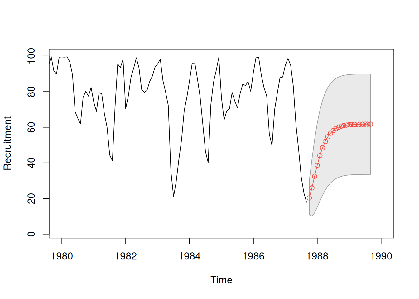
En esta sección se estudian los métodos de estimación de parámetros en procesos ARMA \((p, q)\) causales e invertibles. Se asume que los órdenes \(p\) y \(q\) son conocidos, y se busca estimar los parámetros \(\phi_{1}, \ldots, \phi_{p}\), \(\theta_{1}, \ldots, \theta_{q}\) y \(\sigma_{w}^{2}\). Se presentan los estimadores por momentos (método de Yule-Walker), los de máxima verosimilitud y los de mínimos cuadrados (condicionales e incondicionales), junto con sus propiedades asintóticas y ejemplos ilustrativos.
Para el modelo
\[ x_{t}=\phi_{1}x_{t-1}+\cdots+\phi_{p}x_{t-p}+w_{t}, \]
las ecuaciones de Yule-Walker se definen como:
\[ \gamma(h)=\phi_{1}\gamma(h-1)+\cdots+\phi_{p}\gamma(h-p), \quad h=1,\ldots,p \]
\[ \sigma_{w}^{2}=\gamma(0)-\phi_{1}\gamma(1)-\cdots-\phi_{p}\gamma(p) \]
En forma matricial:
\[ \Gamma_{p}\phi=\gamma_{p}, \quad \sigma_{w}^{2}=\gamma(0)-\phi^{\prime}\gamma_{p}, \]
donde \(\Gamma_{p}={\gamma(k-j)}_{j,k=1}^{p}\), \(\phi=(\phi_{1},\ldots,\phi_{p})^{\prime}\) y \(\gamma_{p}=(\gamma(1),\ldots,\gamma(p))^{\prime}\).
Los estimadores de Yule-Walker se obtienen reemplazando momentos poblacionales por muestrales:
\[ \hat{\phi}=\hat{\Gamma}_{p}^{-1}\hat{\gamma}_{p}, \quad \hat{\sigma}_{w}^{2}=\hat{\gamma}(0)-\hat{\gamma}_{p}^{\prime}\hat{\Gamma}_{p}^{-1}\hat{\gamma}_{p} \]
En términos de la ACF muestral \(\hat{R}_{p}=\{\hat \rho(k-j)\}_{j,k=1}^p\) y asumiendo \(\hat \rho_p=(\hat \rho(1),\ldots,\rho(p))\):
\[ \hat{\phi}=\hat{R}_{p}^{-1}\hat{\rho}_{p}, \quad \hat{\sigma}_{w}^{2}=\hat{\gamma}(0)\left[1-\hat{\rho}_{p}^{\prime}\hat{R}_{p}^{-1}\hat{\rho}_{p}\right]. \]
Propiedad: Resultados asintóticos
Si \(n\to\infty\):
\[ \sqrt{n}(\hat{\phi}-\phi)\xrightarrow{d}N(0,\sigma_{w}^{2}\Gamma_{p}^{-1}), \quad \hat{\sigma}_{w}^{2}\xrightarrow{p}\sigma_{w}^{2}. \]
Propiedad: Distribución del PACF
Para \(h>p\):
\[ \sqrt{n}\,\hat{\phi}_{hh}\xrightarrow{d}N(0,1). \]
Modelo:
\[ x_{t}=1.5x_{t-1}-0.75x_{t-2}+w_{t}, \quad w_{t}\sim N(0,1). \]
Con \(n=144\), se obtuvo:
\[ \hat{\phi}=\binom{1.463}{-0.723}, \quad \hat{\sigma}_{w}^{2}=1.187. \]
Varianzas asintóticas:
\[ \begin{bmatrix} 0.058^{2} & -0.003 \\ -0.003 & 0.058^{2} \end{bmatrix}. \] Código en R:
# Ilustración en R del ejemplo AR(2) con n = 144
# Modelo: x_t = 1.5 x_{t-1} - 0.75 x_{t-2} + w_t,  w_t ~ N(0,1)

set.seed(8675309)  # misma semilla usada en ejemplos clásicos
n <- 144
x <- arima.sim(n = n, list(order = c(2,0,0), ar = c(1.5, -0.75)), sd = 1)

# 1) Estimación Yule-Walker (coeficientes y varianza del error)
fit_yw <- stats::ar.yw(x, order.max = 2, aic = FALSE, demean = TRUE)
phi_hat <- as.numeric(fit_yw$ar)            # (phi1_hat, phi2_hat)
sigma2_hat <- as.numeric(fit_yw$var.pred)   # estimador de sigma_w^2

cat("Coeficientes YW (phi1_hat, phi2_hat):\n")
Coeficientes YW (phi1_hat, phi2_hat):print(round(phi_hat, 3))[1] 1.438 -0.705cat("\nVarianza del ruido (sigma_w^2_hat):\n")
Varianza del ruido (sigma_w^2_hat):print(round(sigma2_hat, 3))[1] 1.327# 2) Matriz Γ_p estimada con autocovarianzas muestrales
# Γ_2 = [[γ(0), γ(1)],
# [γ(1), γ(0)]]
acf_cov <- acf(x, type = "covariance", plot = FALSE)$acf
gamma0_hat <- as.numeric(acf_cov[1]) # γ(0)
gamma1_hat <- as.numeric(acf_cov[2]) # γ(1)
Gamma_hat <- matrix(c(gamma0_hat, gamma1_hat,
gamma1_hat, gamma0_hat), nrow = 2, byrow = TRUE)
# 3) Varianzas asintóticas de (phi1_hat, phi2_hat):
# Var_asint(hat{phi}) ≈ (sigma_w^2_hat / n) * Γ_p^{-1}
asymp_cov <- (sigma2_hat / n) * solve(Gamma_hat)
cat("\nMatriz de varianzas-covarianzas asintótica (~ (sigma_w^2/n) * Γ^{-1}):\n")
Matriz de varianzas-covarianzas asintótica (~ (sigma_w^2/n) * Γ^{-1}):print(round(asymp_cov, 6)) [,1] [,2]
[1,] 0.003566 -0.003007
[2,] -0.003007 0.003566cat("\nComparación con la forma reportada (≈ diag(0.058^2) y off-diag ≈ -0.003):\n")
Comparación con la forma reportada (≈ diag(0.058^2) y off-diag ≈ -0.003):cat("0.058^2 =", round(0.058^2, 6), "\n")0.058^2 = 0.003364 rec.yw = ar.yw(rec, order=2)
rec.yw$x.mean[1] 62.26278rec.yw$ar[1] 1.3315874 -0.4445447sqrt(diag(rec.yw$asy.var.coef))[1] 0.04222637 0.04222637rec.yw$var.pred[1] 94.79912Predicción a 24 pasos:
rec.pr = predict(rec.yw, n.ahead=24)
ts.plot(rec, rec.pr$pred, col=1:2)
lines(rec.pr$pred + rec.pr$se, col=4, lty=2)
lines(rec.pr$pred - rec.pr$se, col=4, lty=2)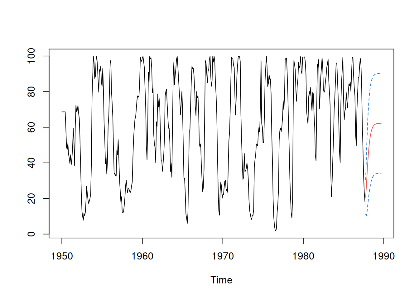
Modelo:
\[ x_{t}=w_{t}+\theta w_{t-1}, \quad |\theta|<1. \]
El estimador de \(\theta\) proviene de:
\[ \hat{\rho}(1)=\frac{\hat{\theta}}{1+\hat{\theta}^{2}}. \]
Solución invertible:
\[ \hat{\theta}=\frac{1-\sqrt{1-4\hat{\rho}(1)^{2}}}{2\hat{\rho}(1)}. \]
Simulación en R:
set.seed(2)
true_rho = 0.9 / (1 + 0.9^2)
ma1 = arima.sim(list(order = c(0,0,1), ma = 0.9), n = 50)
acf(ma1, plot=FALSE)[1]
Autocorrelations of series 'ma1', by lag

    1
0.507 Sea el modelo causal AR(1):
\[ \begin{equation*} x_{t}=\mu+\phi\left(x_{t-1}-\mu\right)+w_{t} \end{equation*} \]
con \(|\phi|<1\) y \(w_{t}\sim \text{iid } \mathrm{N}(0,\sigma_w^2)\). Dado \(x_{1:n}\), la verosimilitud buscada es
\[ L\left(\mu, \phi, \sigma_{w}^{2}\right)=f\left(x_{1}, x_{2}, \ldots, x_{n} \mid \mu, \phi, \sigma_{w}^{2}\right). \]
Para AR(1), usando la factorización condicional:
\[ L\left(\mu, \phi, \sigma_{w}^{2}\right)=f\left(x_{1}\right) f\left(x_{2} \mid x_{1}\right) \cdots f\left(x_{n} \mid x_{n-1}\right), \]
y como \(x_t|x_{t-1}\sim \mathrm{N}\left(\mu+\phi(x_{t-1}-\mu),\sigma_w^2\right)\),
\[ f\left(x_{t} \mid x_{t-1}\right)=f_{w}\left[\left(x_{t}-\mu\right)-\phi\left(x_{t-1}-\mu\right)\right], \]
donde \(f_w\) es la densidad normal de media \(0\) y varianza \(\sigma_w^2\). Entonces:
\[ L\left(\mu, \phi, \sigma_{w}\right)=f\left(x_{1}\right) \prod_{t=2}^{n} f_{w}\left[\left(x_{t}-\mu\right)-\phi\left(x_{t-1}-\mu\right)\right] . \]
Usando la representación causal
\[ x_{1}=\mu+\sum_{j=0}^{\infty} \phi^{j} w_{1-j}, \]
se obtiene \(x_1\sim \mathrm{N}\left(\mu,\ \sigma_w^2/(1-\phi^2)\right)\) y, por tanto, la verosimilitud incondicional es
\[ \begin{equation*} L\left(\mu, \phi, \sigma_{w}^{2}\right)=\left(2 \pi \sigma_{w}^{2}\right)^{-n / 2}\left(1-\phi^{2}\right)^{1 / 2} \exp \left[-\frac{S(\mu, \phi)}{2 \sigma_{w}^{2}}\right] \end{equation*} \]
donde
\[ \begin{equation*} S(\mu, \phi)=\left(1-\phi^{2}\right)\left(x_{1}-\mu\right)^{2}+\sum_{t=2}^{n}\left[\left(x_{t}-\mu\right)-\phi\left(x_{t-1}-\mu\right)\right]^{2}. \end{equation*} \]
Derivando respecto de \(\sigma_w^2\) en el logaritmo de la expresión anterior y anulando, para valores dados de \((\mu,\phi)\) se maximiza con
\[ \begin{equation*} \hat{\sigma}_{w}^{2}=n^{-1} S(\hat{\mu}, \hat{\phi}). \end{equation*} \]
Sustituyendo, el criterio a minimizar en \((\mu,\phi)\) es
\[ \begin{equation*} l(\mu, \phi)=\log \left[n^{-1} S(\mu, \phi)\right]-n^{-1} \log \left(1-\phi^{2}\right). \end{equation*} \]
Condicionando en \(x_1\):
\[ \begin{align*} L\left(\mu, \phi, \sigma_{w}^{2} \mid x_{1}\right) & =\prod_{t=2}^{n} f_{w}\left[\left(x_{t}-\mu\right)-\phi\left(x_{t-1}-\mu\right)\right] \\ & =\left(2 \pi \sigma_{w}^{2}\right)^{-(n-1) / 2} \exp \left[-\frac{S_{c}(\mu, \phi)}{2 \sigma_{w}^{2}}\right], \end{align*} \]
con
\[ \begin{equation*} S_{c}(\mu, \phi)=\sum_{t=2}^{n}\left[\left(x_{t}-\mu\right)-\phi\left(x_{t-1}-\mu\right)\right]^{2}. \end{equation*} \]
El MLE condicional de \(\sigma_w^2\) es
\[ \begin{equation*} \hat{\sigma}_{w}^{2}=S_{c}(\hat{\mu}, \hat{\phi}) /(n-1), \end{equation*} \]
y los MLE condicionales de \((\mu,\phi)\) minimizan \(S_c(\mu,\phi)\). Sea \(\alpha=\mu(1-\phi)\):
\[ \begin{equation*} S_{c}(\mu, \phi)=\sum_{t=2}^{n}\left[x_{t}-\left(\alpha+\phi x_{t-1}\right)\right]^{2}, \end{equation*} \]
lo que es un problema de regresión lineal. De mínimos cuadrados:
\[ \begin{gather*} \hat{\mu}=\frac{\bar{x}_{(2)}-\hat{\phi} \bar{x}_{(1)}}{1-\hat{\phi}}, \\ \hat{\phi}=\frac{\sum_{t=2}^{n}\left(x_{t}-\bar{x}_{(2)}\right)\left(x_{t-1}-\bar{x}_{(1)}\right)}{\sum_{t=2}^{n}\left(x_{t-1}-\bar{x}_{(1)}\right)^{2}}. \end{gather*} \]
En consecuencia, \(\hat{\mu}\approx \bar{x}\) y \(\hat{\phi}\approx \hat{\rho}(1)\); Yule–Walker y MC condicional son cercanos (difieren en el tratamiento de \(x_1\) y \(x_n\)). Puede ajustarse dividiendo por \((n-3)\) en lugar de \((n-1)\) para equivaler a MC.
Para \(\operatorname{ARMA}(p,q)\) normal, con \(\beta=\left(\mu,\phi_{1:p},\theta_{1:q}\right)'\):
\[ L\left(\beta, \sigma_{w}^{2}\right)=\prod_{t=1}^{n} f\left(x_{t} \mid x_{t-1}, \ldots, x_{1}\right), \]
donde \(x_t|x_{t-1:1}\sim \mathrm{N}\left(x_t^{t-1},P_t^{t-1}\right)\) y, recordando el algoritmo de Durbin-Levinson: \(P_t^{t-1}=\gamma(0)\prod_{j=1}^{t-1}(1-\phi_{jj}^2)\). Para ARMA, \(\gamma(0)=\sigma_w^2\sum_{j=0}^\infty \psi_j^2\), así:
\[ P_{t}^{t-1}=\sigma_{w}^{2}\left\{\left[\sum_{j=0}^{\infty} \psi_{j}^{2}\right]\left[\prod_{j=1}^{t-1}\left(1-\phi_{j j}^{2}\right)\right]\right\} \stackrel{\text { def }}{=} \sigma_{w}^{2} r_{t}. \]
La verosimilitud queda
\[ \begin{equation*} L\left(\beta, \sigma_{w}^{2}\right)=\left(2 \pi \sigma_{w}^{2}\right)^{-n / 2}\left[r_{1}(\beta) r_{2}(\beta) \cdots r_{n}(\beta)\right]^{-1 / 2} \exp \left[-\frac{S(\beta)}{2 \sigma_{w}^{2}}\right], \end{equation*} \]
con
\[ \begin{equation*} S(\beta)=\sum_{t=1}^{n}\left[\frac{\left(x_{t}-x_{t}^{t-1}(\beta)\right)^{2}}{r_{t}(\beta)}\right]. \end{equation*} \]
La estimación por MV procede maximizando; como antes:
\[ \begin{equation*} \hat{\sigma}_{w}^{2}=n^{-1} S(\hat{\beta}), \end{equation*} \]
y el criterio concentrado es
\[ \begin{equation*} l(\beta)=\log \left[n^{-1} S(\beta)\right]+n^{-1} \sum_{t=1}^{n} \log r_{t}(\beta). \end{equation*} \]
Para AR(1): \(x_1^0=\mu\), \(x_t^{t-1}=\mu+\phi(x_{t-1}-\mu)\), \(\phi_{11}=\phi\), \(\phi_{hh}=0\) (\(h>1\)), por lo que \(r_1=(1-\phi^2)^{-1}\) y \(r_t=1\) para \(t\ge2\). Así ambas expresiones coinciden; \(S(\beta)\equiv S(\mu,\phi)\) y \(l(\beta)\equiv l(\mu,\phi)\).
Mínimos Cuadrados no condicionales minimiza \(S(\beta)\) en \(\beta\). La Mínimos Cuadrados condicionales también minimiza lo mismo pero condicionando para calcular predicciones/errores; requiere optimización numérica para obtener estimaciones y errores estándar.
Sea \(l(\beta)\) un criterio a minimizar en \(\beta\in\mathbb{R}^k\), p.ej. \(S(\beta)\). Si \(l^{(1)}(\beta)\) son derivadas primeras (vector score) y \(l^{(2)}(\beta)\) la matriz de segundas derivadas (Hessiano):
\[ l^{(1)}(\hat{\beta})=0,\quad l^{(2)}(\beta)=\left\{-\frac{\partial l^{2}(\beta)}{\partial \beta_{i}\partial \beta_{j}}\right\}_{i,j=1}^{k}. \]
Con valor inicial \(\beta_{(0)}\) y expansión de Taylor:
\[ 0\approx l^{(1)}\!\left(\beta_{(0)}\right)-l^{(2)}\!\left(\beta_{(0)}\right)\left[\hat{\beta}-\beta_{(0)}\right], \]
por lo que
\[ \beta_{(1)}=\beta_{(0)}+\left[l^{(2)}\left(\beta_{(0)}\right)\right]^{-1} l^{(1)}\left(\beta_{(0)}\right), \]
iterando hasta converger (Newton–Raphson). En Scoring, se reemplaza \(l^{(2)}(\beta)\) por \(\mathbb{E}[l^{(2)}(\beta)]\) (matriz de información); su inversa aproxima la varianza asintótica de \(\hat{\beta}\).
rec.mle = ar.mle(rec, order=2)
rec.mle$x.mean # 62.26
[1] 62.26153rec.mle$ar # 1.35, -.46[1] 1.3512809 -0.4612736sqrt(diag(rec.mle$asy.var.coef)) # .04, .04[1] 0.04099159 0.04099159rec.mle$var.pred # 89.34[1] 89.33597Modelo en términos de errores para \(\operatorname{ARMA}(p,q)\):
\[ \begin{equation*} w_{t}(\beta)=x_{t}-\sum_{j=1}^{p} \phi_{j} x_{t-j}-\sum_{k=1}^{q} \theta_{k} w_{t-k}(\beta), \end{equation*} \]
destacando la dependencia en \(\beta\).
Mínimos Cuadrados condicionales: condicionar en \(x_{1:p}\) (si \(p>0\)) y en \(w_{p}=w_{p-1}=\dots=w_{1-q}=0\) (si \(q>0\)), y evaluar la ecuación anterior para \(t=p+1,\dots,n\), minimizando
\[ \begin{equation*} S_{c}(\beta)=\sum_{t=p+1}^{n} w_{t}^{2}(\beta). \end{equation*} \]
Si \(q=0\), es regresión lineal; si \(q>0\), es no lineal y requiere optimización.
Mínimos Cuadrados no-condicionales: minimizar \(S(\beta)\), que puede escribirse como
\[ \begin{equation*} S(\beta)=\sum_{t=-\infty}^{n} \tilde{w}_{t}^{2}(\beta), \end{equation*} \]
con \(\tilde{w}_{t}(\beta)=\mathrm{E}(w_t\mid x_{1:n})\); para \(t\le 0\), se obtienen por backcasting. En la práctica se trunca desde \(t=-M+1\) con \(M\) grande.
Gauss–Newton: con inicial \(\beta_{(0)}\), expansión de primer orden
\[ \begin{equation*} w_{t}(\beta) \approx w_{t}\left(\beta_{(0)}\right)-\left(\beta-\beta_{(0)}\right)^{\prime} z_{t}\left(\beta_{(0)}\right), \end{equation*} \]
donde
\[ z_{t}^{\prime}\left(\beta_{(0)}\right)=\left.\left(-\frac{\partial w_{t}(\beta)}{\partial \beta_{1}}, \ldots,-\frac{\partial w_{t}(\beta)}{\partial \beta_{p+q}}\right)\right|_{\beta=\beta_{(0)}}. \]
La aproximación lineal de \(S_c(\beta)\) es
\[ \begin{equation*} Q(\beta)=\sum_{t=p+1}^{n}\left[w_{t}\left(\beta_{(0)}\right)-\left(\beta-\beta_{(0)}\right)^{\prime} z_{t}\left(\beta_{(0)}\right)\right]^{2}. \end{equation*} \]
El estimador de un paso que minimiza \(Q(\beta)\) es
\[ \begin{align*} \left(\widehat{\beta-\beta_{(0)}}\right)&=\left(n^{-1} \sum_{t=p+1}^{n} z_{t}\left(\beta_{(0)}\right) z_{t}^{\prime}\left(\beta_{(0)}\right)\right)^{-1}\left(n^{-1} \sum_{t=p+1}^{n} z_{t}\left(\beta_{(0)}\right) w_{t}\left(\beta_{(0)}\right)\right)\\ &=:\Delta\left(\beta_{(0)}\right). \end{align*} \]
y se itera
\[ \begin{equation*} \beta_{(1)}=\beta_{(0)}+\Delta\left(\beta_{(0)}\right), \end{equation*} \]
con \(\beta_{(j)}=\beta_{(j-1)}+\Delta(\beta_{(j-1)})\) hasta convergencia.
Para \(x_t=w_t+\theta w_{t-1}\) (invertible), los errores truncados:
\[ \begin{equation*} w_{t}(\theta)=x_{t}-\theta w_{t-1}(\theta), \quad t=1, \ldots, n \end{equation*} \]
con \(w_0(\theta)=0\). Derivando e igualando a cero:
\[ \begin{equation*} -\frac{\partial w_{t}(\theta)}{\partial \theta}=w_{t-1}(\theta)+\theta \frac{\partial w_{t-1}(\theta)}{\partial \theta}, \quad t=1, \ldots, n \end{equation*} \]
equivalentemente
\[ \begin{equation*} z_{t}(\theta)=w_{t-1}(\theta)-\theta z_{t-1}(\theta), \quad t=1, \ldots, n, \end{equation*} \]
con \(z_t(\theta)=-\partial w_t(\theta)/\partial \theta\) y \(z_0(\theta)=0\). El paso iterativo:
\[ \begin{equation*} \theta_{(j+1)}=\theta_{(j)}+\frac{\sum_{t=1}^{n} z_{t}\left(\theta_{(j)}\right) w_{t}\left(\theta_{(j)}\right)}{\sum_{t=1}^{n} z_{t}^{2}\left(\theta_{(j)}\right)}, \quad j=0,1,2, \ldots \end{equation*} \]
se detiene cuando \(|\theta_{(j+1)}-\theta_{(j)}|\) o \(|Q(\theta_{(j+1)})-Q(\theta_{(j)})|\) es pequeño.
Transformación y diferencia:
\[ \nabla \log(x_t)=\log(x_t)-\log(x_{t-1})=\log\!\left(\frac{x_t}{x_{t-1}}\right), \]
x = diff(log(varve))
acf2(x)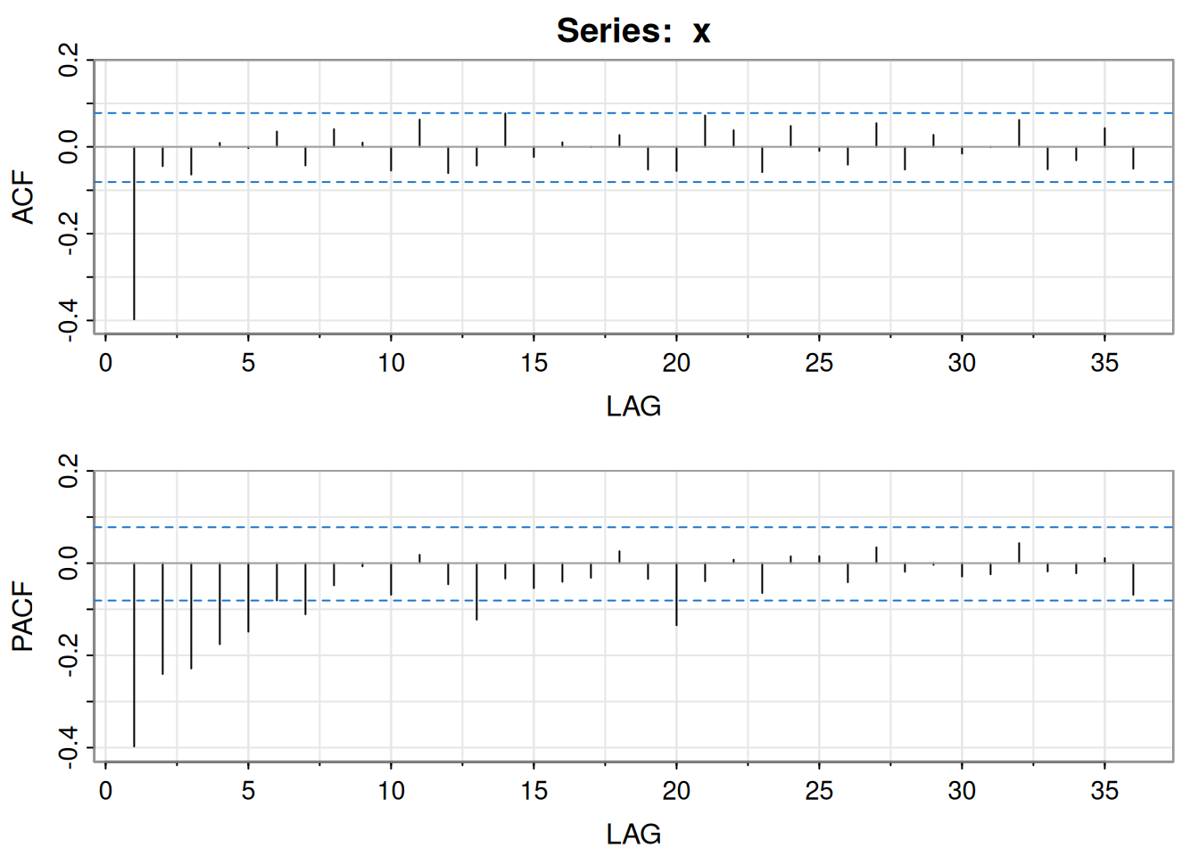
     [,1]  [,2]  [,3]  [,4]  [,5]  [,6]  [,7]  [,8]  [,9] [,10] [,11] [,12]
ACF  -0.4 -0.04 -0.06  0.01  0.00  0.04 -0.04  0.04  0.01 -0.05  0.06 -0.06
PACF -0.4 -0.24 -0.23 -0.18 -0.15 -0.08 -0.11 -0.05 -0.01 -0.07  0.02 -0.05
     [,13] [,14] [,15] [,16] [,17] [,18] [,19] [,20] [,21] [,22] [,23] [,24]
ACF  -0.04  0.08 -0.02  0.01  0.00  0.03 -0.05 -0.06  0.07  0.04 -0.06  0.05
PACF -0.12 -0.03 -0.05 -0.04 -0.03  0.03 -0.03 -0.13 -0.04  0.01 -0.06  0.01
     [,25] [,26] [,27] [,28] [,29] [,30] [,31] [,32] [,33] [,34] [,35] [,36]
ACF  -0.01 -0.04  0.05 -0.05  0.03 -0.02  0.00  0.06 -0.05 -0.03  0.04 -0.05
PACF  0.02 -0.04  0.03 -0.02  0.00 -0.03 -0.02  0.04 -0.02 -0.02  0.01 -0.07
lo cual sugiere MA(1).
Con \(\hat{\rho}(1)=-0.397\), el inicial por mínimos cuadrados es \(\theta_{(0)}=-0.495\).
Código utilizado:
# Evaluate Sc on a Grid
c(0) -> w -> z
c() -> Sc -> Sz -> Szw
num = length(x)
th = seq(-.3,-.94,-.01)
for (p in 1:length(th)){
        for (i in 2:num){ w[i] = x[i]-th[p]*w[i-1] }
            Sc[p] = sum(w^2) }
plot(th, Sc, type="l", ylab=expression(S[c](theta)), xlab=expression(theta),
                lwd=2)
# Gauss-Newton Estimation
r = acf(x, lag=1, plot=FALSE) $acf[-1]
rstart = (1-sqrt(1-4*(r^2)))/(2*r) # from (3.105)
c(0) -> w -> z
c() -> Sc -> Sz -> Szw -> para
niter = 12
para[1] = rstart
for (p in 1:niter){
        for (i in 2:num){ w[i] = x[i]-para[p]*w[i-1]
                    z[i] = w[i-1]-para[p]*z[i-1] }
        Sc[p] = sum(w^2)
        Sz[p] = sum(z^2)
        Szw[p] = sum(z*w)
        para[p+1] = para[p] + Szw[p]/Sz[p] }
round(cbind(iteration=0:(niter-1), thetahat=para[1:niter], Sc, Sz ), 3)
iteration thetahat Sc Sz
[1,] 0 -0.495 158.739 171.240
[2,] 1 -0.668 150.747 235.266
[3,] 2 -0.733 149.264 300.562
[4,] 3 -0.756 149.031 336.823
[5,] 4 -0.766 148.990 354.173
[6,] 5 -0.769 148.982 362.167
[7,] 6 -0.771 148.980 365.801
[8,] 7 -0.772 148.980 367.446
[9,] 8 -0.772 148.980 368.188
[10,] 9 -0.772 148.980 368.522
[11,] 10 -0.773 148.980 368.673
[12,] 11 -0.773 148.980 368.741abline(v = para[1:12], lty=2)
points(para[1:12], Sc[1:12], pch=16)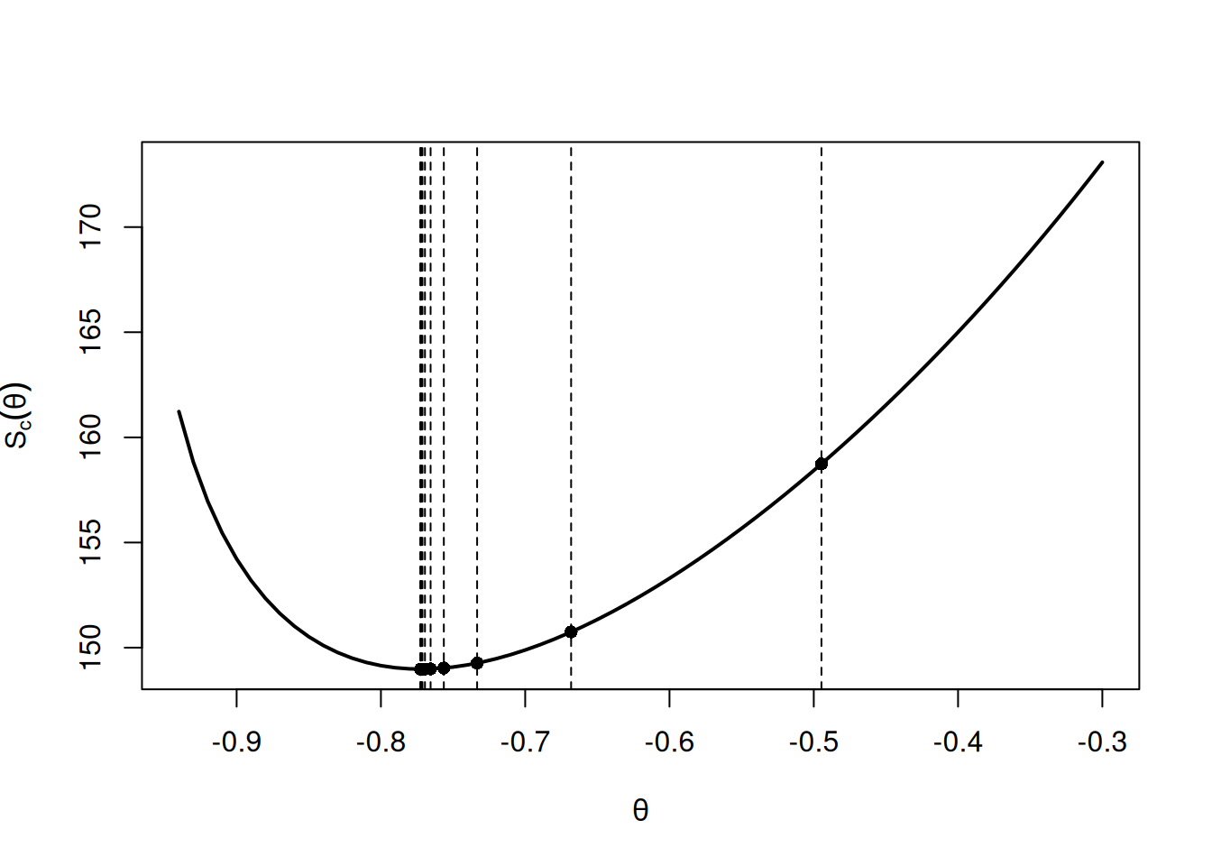
Tabla 3.2. Resultados Gauss–Newton (extracto):
| \(j\) | \(\theta_{(j)}\) | \(S_{c}\left(\theta_{(j)}\right)\) | \(\sum_{t=1}^{n} z_{t}^{2}\left(\theta_{(j)}\right)\) |
|---|---|---|---|
| 0 | -0.495 | 158.739 | 171.240 |
| 1 | -0.668 | 150.747 | 235.266 |
| 2 | -0.733 | 149.264 | 300.562 |
| 3 | -0.756 | 149.031 | 336.823 |
| 4 | -0.766 | 148.990 | 354.173 |
| 5 | -0.769 | 148.982 | 362.167 |
| 6 | -0.771 | 148.980 | 365.801 |
| 7 | -0.772 | 148.980 | 367.446 |
| 8 | -0.772 | 148.980 | 368.188 |
| 9 | -0.772 | 148.980 | 368.522 |
| 10 | -0.773 | 148.980 | 368.673 |
| 11 | -0.773 | 148.980 | 368.741 |
Tras 11 iteraciones de Gauss–Newton, \(\hat{\theta}=\theta_{(11)}=-0.773\), con \(S_c(\theta)=148.98\), \(\hat{\sigma}*w^2=148.98/632=0.236\) (632 g.l.) y \(\sum z_t^2(\theta*{(11)})=368.741\), por lo que \(se(\hat{\theta})=\sqrt{0.236/368.741}=0.025\) y \(t=-30.92\).
Propiedad: Distribución asintótica de los estimadores
Bajo condiciones apropiadas y ARMA causal e invertible, los MLE, MC incondicional y MC condicional (inicializados por momentos) son óptimos: \(\hat{\sigma}_w^2\) consistente y
\[ \begin{equation*} \sqrt{n}(\hat{\beta}-\beta) \xrightarrow{d} N\left(0, \sigma_{w}^{2} \Gamma_{p, q}^{-1}\right). \end{equation*} \]
La matriz de información \((p+q)\times(p+q)\) es
\[ \Gamma_{p, q}=\left(\begin{array}{cc} \Gamma_{\phi \phi} & \Gamma_{\phi \theta} \\ \Gamma_{\theta \phi} & \Gamma_{\theta \theta} \end{array}\right), \]
donde \(\Gamma_{\phi\phi}\) tiene entradas \(\gamma_x(i-j)\) del AR(\(p\)) \(\phi(B)x_t=w_t\), \(\Gamma_{\theta\theta}\) tiene entradas \(\gamma_y(i-j)\) del AR(\(q\)) \(\theta(B)y_t=w_t\), y \(\Gamma_{\phi\theta}\) tiene entradas de covarianza cruzada \(\gamma_{xy}(i-j)\) entre esos procesos; \(\Gamma_{\theta\phi}=\Gamma_{\phi\theta}'\).
AR(1): \(\gamma_x(0)=\sigma_w^2/(1-\phi^2)\), por lo que
\[ \begin{equation*} \hat{\phi} \sim \operatorname{AN}\left[\phi, \ n^{-1}\left(1-\phi^{2}\right)\right]. \end{equation*} \]
AR(2): Con
\[ \gamma_{x}(0)=\left(\frac{1-\phi_{2}}{1+\phi_{2}}\right) \frac{\sigma_{w}^{2}}{\left(1-\phi_{2}\right)^{2}-\phi_{1}^{2}},\quad \gamma_x(1)=\phi_1\gamma_x(0)+\phi_2\gamma_x(1), \]
se obtiene
\[ \binom{\hat{\phi}_{1}}{\hat{\phi}_{2}} \sim \operatorname{AN}\left[\binom{\phi_{1}}{\phi_{2}}, \ n^{-1}\left(\begin{array}{cc} 1-\phi_{2}^{2} & -\phi_{1}\left(1+\phi_{2}\right) \\ \operatorname{sym} & 1-\phi_{2}^{2} \end{array}\right)\right] . \]
MA(1): Con \(\theta(B) y_{t}=w_{t}\) (\(y_t+\theta y_{t-1}=w_t\)), análogo a AR(1),
\[ \begin{equation*} \hat{\theta} \sim \operatorname{AN}\left[\theta, \ n^{-1}\left(1-\theta^{2}\right)\right]. \end{equation*} \]
MA(2):
\[ \binom{\hat{\theta}_{1}}{\hat{\theta}_{2}} \sim \operatorname{AN}\left[\binom{\theta_{1}}{\theta_{2}}, \ n^{-1}\left(\begin{array}{cc} 1-\theta_{2}^{2} & \theta_{1}\left(1+\theta_{2}\right)\\ \operatorname{sym} & 1-\theta_{2}^{2} \end{array}\right)\right] . \]
ARMA(1,1): Con \(x_t-\phi x_{t-1}=w_t\) y \(y_t+\theta y_{t-1}=w_t\),
\[ \begin{aligned} \gamma_{x y}(0) & =\operatorname{cov}\left(x_{t}, y_{t}\right)=\operatorname{cov}\left(\phi x_{t-1}+w_{t},-\theta y_{t-1}+w_{t}\right) \\ & =-\phi \theta \gamma_{x y}(0)+\sigma_{w}^{2} \end{aligned} \]
de donde \(\gamma_{xy}(0)=\sigma_w^2/(1+\phi\theta)\) y
\[ \binom{\hat{\phi}}{\hat{\theta}} \sim \operatorname{AN}\left[\binom{\phi}{\theta}, \ n^{-1}\left[\begin{array}{cc} \left(1-\phi^{2}\right)^{-1} & (1+\phi \theta)^{-1} \\ \text { sym } & \left(1-\theta^{2}\right)^{-1} \end{array}\right]^{-1}\right]. \]
Nota: Si el verdadero proceso es AR(1) y se ajusta AR(2), la varianza de \(\hat{\phi}_1\) aumenta: ajustando AR(1), \(\operatorname{var}(\hat{\phi}_1)\approx n^{-1}(1-\phi_1^2)\); ajustando AR(2) a un AR(1), \(\phi_2=0\) y \(\operatorname{var}(\hat{\phi}_1)\approx n^{-1}\) (inflación).
Modelo:
\[ \begin{equation*} x_{t}=\mu+\phi\left(x_{t-1}-\mu\right)+w_{t}, \quad \mu=50,\ \phi=0.95, \end{equation*} \]
con \(w_t\) iid Laplace(0, \(\beta=2\)), densidad
\[ f(w)=\frac{1}{2 \beta} \exp \{-|w| / \beta\}, \quad \mathbb{E}(w_t)=0,\ \operatorname{var}(w_t)=2\beta^2=8. \]
Simulación de 100 observaciones (aparentan no estacionariedad pero el modelo es estacionario y no normal):
set.seed(101010)
e = rexp(150, rate=.5); u = runif(150,-1,1); de = e*sign(u)
dex = 50 + arima.sim(n=100, list(ar=.95), innov=de, n.start=50)
plot.ts(dex, type='o', ylab=expression(X[~t]))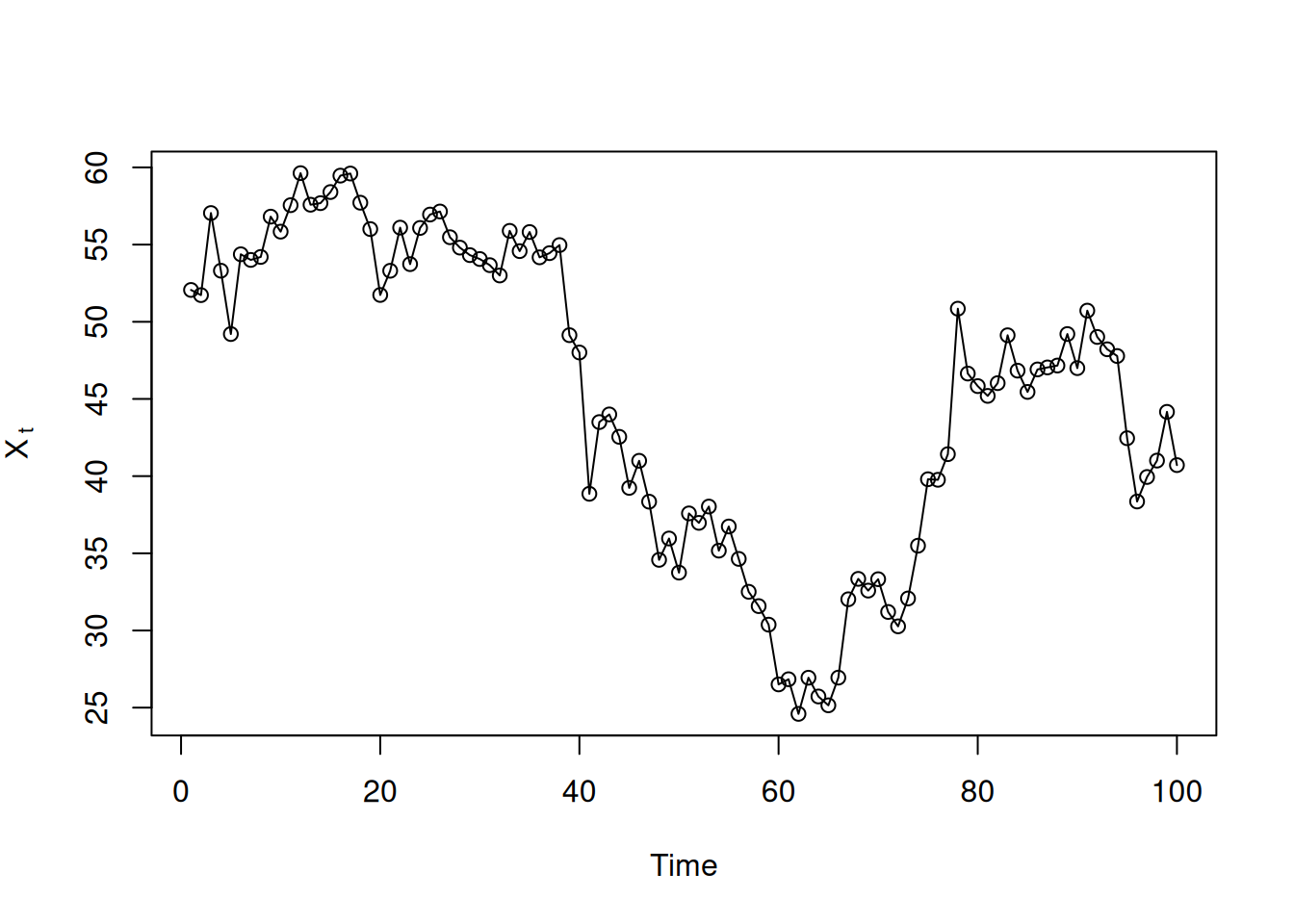
Estimación Yule–Walker en estos datos:
fit = ar.yw(dex, order=1)
round(cbind(fit$x.mean, fit$ar, fit$var.pred), 2)
[,1] [,2] [,3]
[1,] 45.25 0.96 7.88Simulación para aproximar la distribución finita muestral de \(\hat{\phi}\) (1000 réplicas):
set.seed(111)
phi.yw = rep(NA, 1000)
for (i in 1:1000){
    e = rexp(150, rate=.5); u = runif(150,-1,1); de = e*sign(u)
    x = 50 + arima.sim(n=100,list(ar=.95), innov=de, n.start=50)
    phi.yw[i] = ar.yw(x, order=1)$ar }
Bootstrap condicional en \(x_1\) con innovaciones empíricas: Los predictores de un paso:
\[ x_{t}^{t-1}=\mu+\phi\left(x_{t-1}-\mu\right),\quad t=2,\dots,100, \]
innovaciones
\[ \begin{equation*} \epsilon_{t}=\left(x_{t}-\mu\right)-\phi\left(x_{t-1}-\mu\right), \quad t=2, \ldots, 100, \end{equation*} \]
y el modelo en innovaciones:
\[ \begin{equation*} x_{t}=x_{t}^{t-1}+\epsilon_{t}=\mu+\phi\left(x_{t-1}-\mu\right)+\epsilon_{t}. \end{equation*} \]
Sustituyendo \(\hat{\mu}=45.25\), \(\hat{\phi}=0.96\), muestreando con reemplazo \({\hat{\epsilon}_2,\dots,\hat{\epsilon}_{100}}\) y generando
\[ \begin{equation*} x_{t}^{*}=45.25+.96\left(x_{t-1}^{*}-45.25\right)+\epsilon_{t}^{*}, \quad t=2, \ldots, 100, \end{equation*} \]
con \(x_1^*=x_1\), se reestima para obtener \({\hat{\phi}(b)}_{b=1}^B\).
Código de bootstrap y visualización:
set.seed(666) # not that 666
fit = ar.yw(dex, order=1) # assumes the data were retained
m = fit$x.mean # estimate of mean
phi = fit$ar # estimate of phi
nboot = 500 # number of bootstrap replicates
resids = fit$resid[-1] # the 99 innovations
x.star = dex # initialize x*
phi.star.yw = rep(NA, nboot)
# Bootstrap
for (i in 1:nboot) {
resid.star = sample(resids, replace=TRUE)
    for (t in 1:99){ x.star[t+1] = m + phi*(x.star[t]-m) + resid.star[t] }
    phi.star.yw[i] = ar.yw(x.star, order=1)$ar
}
# Picture
culer = rgb(.5,.7,1,.5)
hist(phi.star.yw, 15, main="", prob=TRUE, xlim=c(.65,1.05), ylim=c(0,14),
    col=culer, xlab=expression(hat(phi)))
lines(density(phi.yw, bw=.02), lwd=2) # from previous simulation
u = seq(.75, 1.1, by=.001) # normal approximation
lines(u, dnorm(u, mean=.96, sd=.03), lty=2, lwd=2)
legend(.65, 14, legend=c('true distribution', 'bootstrap distribution',
    'normal approximation'), bty='n', lty=c(1,0,2), lwd=c(2,0,2),
    col=1, pch=c(NA,22,NA), pt.bg=c(NA,culer,NA), pt.cex=2.5)
Se extiende ARMA a modelos integrados ARIMA para manejar no estacionariedad mediante diferenciación. Se muestran casos determinísticos y estocásticos de tendencia que se vuelven estacionarios al diferenciar el orden adecuado. Se define ARIMA\((p,d,q)\), se comenta el cálculo de pronósticos y sus errores, y se ilustran dos ejemplos: la caminata aleatoria con drift y el IMA(1,1) vinculado con EWMA.
Sea \(x_t\) una caminata aleatoria \(x_t=x_{t-1}+w_t\); al diferenciar:
\[ \nabla x_{t}=w_{t} \]
es estacionaria. En muchas series, \(x_t\) se compone de una tendencia no estacionaria y un componente estacionario de media cero:
\[ \begin{equation*} x_{t}=\mu_{t}+y_{t}, \end{equation*} \]
donde \(\mu_t=\beta_0+\beta_1 t\) y \(y_t\) es estacionaria. Diferenciando:
\[ \nabla x_{t}=x_{t}-x_{t-1}=\beta_{1}+y_{t}-y_{t-1}=\beta_{1}+\nabla y_{t}. \]
Si \(\mu_t\) es estocástica y varía lentamente como una caminata aleatoria, \(\mu_t=\mu_{t-1}+v_t\) con \(v_t\) estacionaria, entonces:
\[ \nabla x_{t}=v_{t}+\nabla y_{t} \]
es estacionaria. Si \(\mu_t\) es un polinomio de orden \(k\), \(\mu_t=\sum_{j=0}^{k}\beta_j t^j\), entonces (Problema 3.27) \(\nabla^k x_t\) es estacionaria. Para tendencias estocásticas de mayor orden, por ejemplo:
\[ \mu_{t}=\mu_{t-1}+v_{t}\quad \text{y}\quad v_{t}=v_{t-1}+e_{t}, \]
con \(e_t\) estacionaria, se tiene que \(\nabla x_t=v_t+\nabla y_t\) no es estacionaria, pero
\[ \nabla^{2} x_{t}=e_{t}+\nabla^{2} y_{t} \]
sí lo es.
El modelo ARIMA amplía ARMA incluyendo diferenciación.
Definición 3.11. Un proceso \(x_t\) es ARIMA\((p,d,q)\) si
\[ \nabla^{d} x_{t}=(1-B)^{d} x_{t} \]
es ARMA\((p,q)\). En general:
\[ \begin{equation*} \phi(B)(1-B)^{d} x_{t}=\theta(B) w_{t}. \tag{3.144} \end{equation*} \]
Si \(\mathrm{E}(\nabla^{d}x_t)=\mu\), se escribe
\[ \phi(B)(1-B)^{d} x_{t}=\delta+\theta(B) w_{t}, \]
donde \(\delta=\mu(1-\phi_1-\cdots-\phi_p)\).
Sea \(y_t=\nabla^{d}x_t\) (ARMA). Usando los métodos de la Sección 3.5 se pronostica \(y_t\) y, para \(d=1\), se reconstruye \(x_t\) vía:
\[ x_{n+m}^{n}=y_{n+m}^{n}+x_{n+m-1}^{n}, \]
con condición inicial \(x_{n+1}^{n}=y_{n+1}^{n}+x_n\) (y \(x_n^n=x_n\)).
Para el error de predicción, para \(n\) grande, se aproxima por:
\[ \begin{equation*} P_{n+m}^{n}=\sigma_{w}^{2} \sum_{j=0}^{m-1} \psi_{j}^{* 2}, \end{equation*} \]
donde \(\psi_{j}^{*}\) es el coeficiente de \(z^j\) en \(\psi^{*}(z)=\theta(z)/{\phi(z)(1-z)^{d}}\).
Modelo:
\[ x_{t}=\delta+x_{t-1}+w_{t},\quad t=1,2,\ldots,\ \ x_0=0. \]
(ARIMA\((0,1,0)\) con drift). El pronóstico a un paso:
\[ x_{n+1}^{n}=\mathrm{E}(x_{n+1}\mid x_{1:n})=\delta+x_n. \]
A dos pasos \(x_{n+2}^{n}=\delta+x_{n+1}^{n}=2\delta+x_n\), y en general:
\[ \begin{equation*} x_{n+m}^{n}=m \delta+x_{n}. \end{equation*} \]
Usando \(x_n=n\delta+\sum_{j=1}^{n}w_j\):
\[ x_{n+m}=(n+m)\delta+\sum_{j=1}^{n+m}w_j=m\delta+x_n+\sum_{j=n+1}^{n+m}w_j, \]
por lo que el MSPE es
\[ \begin{equation*} P_{n+m}^{n}=\mathrm{E}\!\left(x_{n+m}-x_{n+m}^{n}\right)^{2} =\mathrm{E}\!\left(\sum_{j=n+1}^{n+m}w_j\right)^{2} =m\sigma_w^2. \end{equation*} \]
Bajo gaussianidad, la estimación es directa ya que \(y_t=\nabla x_t\) son iid \(\mathrm{N}(\delta,\sigma_w^2)\); los estimadores óptimos de \(\delta\) y \(\sigma_w^2\) son la media y varianza muestral de \(y_t\).
Modelo ARIMA\((0,1,1)\) (IMA\((1,1)\)):
\[ \begin{equation*} x_{t}=x_{t-1}+w_{t}-\lambda w_{t-1}, \end{equation*} \]
con \(|\lambda|<1\), \(t\ge1\), \(x_0=0\) (sin drift para simplificar). Definiendo
\[ y_t=w_t-\lambda w_{t-1}, \]
se tiene \(x_t=x_{t-1}+y_t\). Como \(|\lambda|<1\), \(y_t\) es invertible: \(y_t=\sum_{j=1}^{\infty}\lambda^j y_{t-j}+w_t\). Sustituyendo \(y_t=x_t-x_{t-1}\) y tomando \(x_t=0\) para \(t\le0\), se obtiene la aproximación (para \(t\) grande):
\[ \begin{equation*} x_{t}=\sum_{j=1}^{\infty}(1-\lambda)\lambda^{j-1}x_{t-j}+w_t. \end{equation*} \]
El predictor aproximado a un paso:
\[ \begin{align*} \tilde{x}_{n+1} &=\sum_{j=1}^{\infty}(1-\lambda)\lambda^{j-1}x_{n+1-j} \\ &=(1-\lambda)x_n+\lambda \sum_{j=1}^{\infty}(1-\lambda)\lambda^{j-1}x_{n-j}\\ &=(1-\lambda)x_n+\lambda \tilde{x}_n. \end{align*} \]
Con datos observados \(x_{1:n}\) (y \(y_{1:n}\)), los pronósticos truncados cumplen:
\[ \begin{equation*} \tilde{x}_{n+1}^{n}=(1-\lambda)x_n+\lambda \tilde{x}_{n}^{\,n-1},\quad n\ge1, \end{equation*} \]
con \(\tilde{x}_1^{0}=x_1\) inicial. El MSPE aproximado (\(\psi^{*}(z)=(1-\lambda z)/(1-z)=1+(1-\lambda)\sum_{j=1}^{\infty}z^j\)) es, para \(n\) grande:
\[ P_{n+m}^{n}\approx \sigma_w^2\left[1+(m-1)(1-\lambda)^2\right]. \]
En EWMA, \(1-\lambda\) es el parámetro de suavizamiento (entre 0 y 1); \(\lambda\) mayor implica mayor suavidad. Es un método popular por su simplicidad, aunque a veces mal usado si no se verifica el IMA\((1,1)\) ni se elige \(\lambda\) apropiadamente.
Código R (simulación IMA\((1,1)\) con \(\lambda=-\theta=0.8\) y ajuste EWMA vía Holt–Winters):
set.seed(666)
x = arima.sim(list(order = c(0,1,1), ma = -0.8), n = 100)
(x.ima = HoltWinters(x, beta=FALSE, gamma=FALSE)) # \alpha below is 1-\lambda
Holt-Winters exponential smoothing without trend and without seasonal component.
Call:
HoltWinters(x = x, beta = FALSE, gamma = FALSE)
Smoothing parameters:
alpha: 0.1663072
beta : FALSE
gamma: FALSE
Coefficients:
[,1]
a -2.241533plot(x.ima)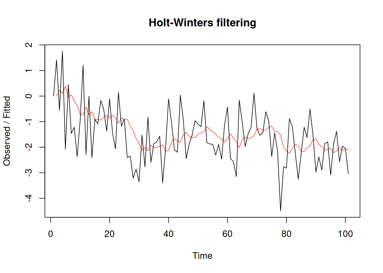
Smoothing parameter: alpha: 0.1663072
Esta sección describe el flujo de trabajo para construir modelos ARIMA: graficar y transformar los datos si es necesario, identificar órdenes \((p,d,q)\) mediante inspección de gráficos y funciones de autocorrelación, estimar parámetros, realizar diagnósticos y elegir el modelo final. Se ilustra con ejemplos sobre el PIB trimestral de EE. UU. (GNP), diagnósticos de residuales, un caso de sobreajuste y la selección de modelos por AIC, AICc y BIC.
Datos trimestrales (1947(1)–2002(3), \(n=223\)), GNP real (dólares 1996, ajustado por estacionalidad). Sea \(y_t\) el GNP y \(x_t=\nabla\log(y_t)\) su tasa de crecimiento (aparenta ser estable).
A partir de ACF/PACF del crecimiento trimestral: posible MA(2) para \(x_t\) \(\Rightarrow\) \(\log y_t\) es \(\operatorname{ARIMA}(0,1,2)\); alternativamente, ACF que decae y PACF con corte en 1 sugiere AR(1) para \(x_t\) \(\Rightarrow\) \(\operatorname{ARIMA}(1,1,0)\) para \(\log y_t\).
MA(2) (MLE) para \(x_t\):
\[ \hat{x}_t=.008_{(.001)}+.303_{(.065)}\hat w_{t-1}+.204_{(.064)}\hat w_{t-2}+\hat w_t, \]
con \(\hat\sigma_w=.0094\) (219 g.l.). Todos los coeficientes, incluida la constante, son significativos.
AR(1) para \(x_t\):
\[ \hat{x}_t=.008_{(.001)}(1-.347)+.347_{(.063)}\hat x_{t-1}+\hat w_t, \]
con \(\hat\sigma_w=.0095\) (220 g.l.). La constante es \(.008(1-.347)=.005\).
Equivalencia aproximada AR(1) ↔︎ MA(2): si \(x_t=.35x_{t-1}+w_t\), su forma causal \(x_t=\sum_{j\ge0}\psi_j w_{t-j}\) tiene \(\psi_j=.35^j\), de modo que
\[ x_t\approx .35\,w_{t-1}+.12\,w_{t-2}+w_t, \]
similar al MA(2) ajustado.
# Análisis en R (según el texto)
plot(gnp)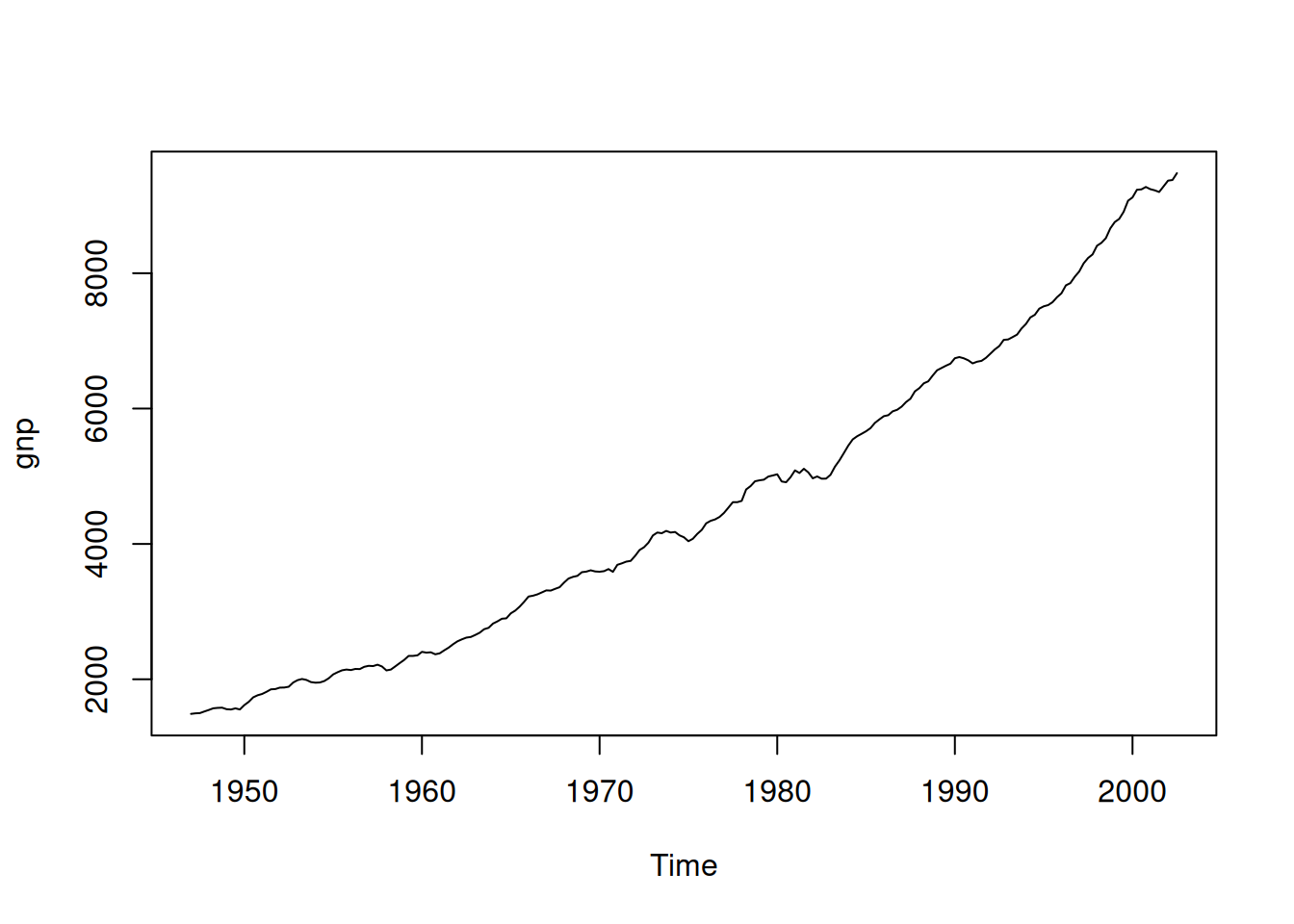
acf2(gnp, 50)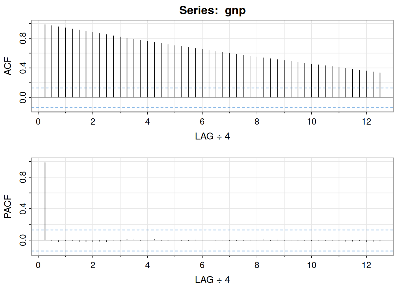
     [,1] [,2]  [,3] [,4] [,5]  [,6]  [,7]  [,8]  [,9] [,10] [,11] [,12] [,13]
ACF  0.99 0.97  0.96 0.94 0.93  0.91  0.90  0.88  0.87  0.85  0.83  0.82  0.80
PACF 0.99 0.00 -0.02 0.00 0.00 -0.02 -0.02 -0.02 -0.01 -0.02  0.00 -0.01  0.01
     [,14] [,15] [,16] [,17] [,18] [,19] [,20] [,21] [,22] [,23] [,24] [,25]
ACF   0.79  0.77  0.76  0.74  0.73  0.72   0.7  0.69  0.68  0.66  0.65  0.64
PACF  0.00  0.00  0.00  0.01  0.00 -0.01   0.0 -0.01 -0.01  0.00  0.00  0.00
     [,26] [,27] [,28] [,29] [,30] [,31] [,32] [,33] [,34] [,35] [,36] [,37]
ACF   0.62  0.61  0.60  0.59  0.57  0.56  0.55  0.54  0.52  0.51   0.5  0.49
PACF -0.01  0.00 -0.01 -0.01 -0.01 -0.01 -0.01  0.00 -0.01  0.00   0.0  0.00
     [,38] [,39] [,40] [,41] [,42] [,43] [,44] [,45] [,46] [,47] [,48] [,49]
ACF   0.48  0.47  0.45  0.44  0.43  0.42  0.41  0.40  0.38  0.37  0.36  0.35
PACF -0.01 -0.01 -0.01  0.00 -0.01 -0.01 -0.01 -0.01 -0.01 -0.01 -0.02 -0.02
     [,50]
ACF   0.33
PACF -0.01
gnpgr = diff(log(gnp)) # growth rate
plot(gnpgr)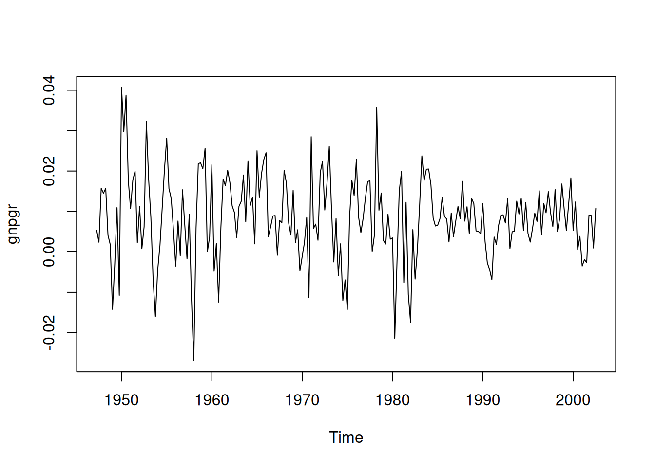
acf2(gnpgr, 24)
     [,1] [,2]  [,3]  [,4]  [,5]  [,6]  [,7]  [,8] [,9] [,10] [,11] [,12] [,13]
ACF  0.35 0.19 -0.01 -0.12 -0.17 -0.11 -0.09 -0.04 0.04  0.05  0.03 -0.12 -0.13
PACF 0.35 0.08 -0.11 -0.12 -0.09  0.01 -0.03 -0.02 0.05  0.01 -0.03 -0.17 -0.06
     [,14] [,15] [,16] [,17] [,18] [,19] [,20] [,21] [,22] [,23] [,24]
ACF  -0.10 -0.11  0.05  0.07  0.10  0.06  0.07 -0.09 -0.05 -0.10 -0.05
PACF 0.02 -0.06 0.10 0.00 0.02 -0.04 0.01 -0.11 0.03 -0.03 0.00sarima(gnpgr, 1, 0, 0) # AR(1)initial value -4.589567
iter 2 value -4.654150
iter 3 value -4.654150
iter 4 value -4.654151
iter 4 value -4.654151
iter 4 value -4.654151
final value -4.654151
converged
initial value -4.655919
iter 2 value -4.655921
iter 3 value -4.655922
iter 4 value -4.655922
iter 5 value -4.655922
iter 5 value -4.655922
iter 5 value -4.655922
final value -4.655922
converged
<><><><><><><><><><><><><><>
Coefficients:
Estimate SE t.value p.value
ar1 0.3467 0.0627 5.5255 0
xmean 0.0083 0.0010 8.5398 0
sigma^2 estimated as 9.029569e-05 on 220 degrees of freedom
AIC = -6.44694 AICc = -6.446693 BIC = -6.400958

sarima(gnpgr, 0, 0, 2) # MA(2)initial value -4.591629
iter 2 value -4.661095
iter 3 value -4.662220
iter 4 value -4.662243
iter 5 value -4.662243
iter 6 value -4.662243
iter 6 value -4.662243
iter 6 value -4.662243
final value -4.662243
converged
initial value -4.662022
iter 2 value -4.662023
iter 2 value -4.662023
iter 2 value -4.662023
final value -4.662023
converged
<><><><><><><><><><><><><><>
Coefficients:
Estimate SE t.value p.value
ma1 0.3028 0.0654 4.6272 0.0000
ma2 0.2035 0.0644 3.1594 0.0018
xmean 0.0083 0.0010 8.7178 0.0000
sigma^2 estimated as 8.919178e-05 on 219 degrees of freedom
AIC = -6.450133 AICc = -6.449637 BIC = -6.388823

ARMAtoMA(ar=.35, ma=0, 10) # imprime pesos psi [1] 3.500000e-01 1.225000e-01 4.287500e-02 1.500625e-02 5.252187e-03
[6] 1.838266e-03 6.433930e-04 2.251875e-04 7.881564e-05 2.758547e-05Sea \(\hat x_t^{t-1}\) el predictor a un paso y \(\hat P_t^{t-1}\) su varianza estimada. Residuales (innovaciones) estandarizados:
\[ e_t=\frac{x_t-\hat x_t^{\,t-1}}{\sqrt{\hat P_t^{\,t-1}}}. \]
\[ Q=n(n+2)\sum_{h=1}^{H}\frac{\hat\rho_e^2(h)}{n-h}, \]
con \(H\) típico \(=20\); bajo \(H_0\) (adecuación del modelo), asintóticamente \(Q\sim\chi^2_{H-p-q}\). Rechazar si \(Q>\chi^2_{H-p-q,,1-\alpha}\).
Se ajustó \(\operatorname{ARIMA}(0,1,1)\) a \(\log(\text{varve})\); quedan autocorrelaciones en residuales y los Q-tests son significativos. Ajustando \(\operatorname{ARIMA}(1,1,1)\):
\[ \hat\phi=.23_{(.05)},\quad \hat\theta=-.89_{(.03)},\quad \hat\sigma_w^2=.23. \]
El término AR es significativo y los p-valores del \(Q\) indican buen ajuste.
# Código R del texto
sarima(log(varve), 0, 1, 1, no.constant=TRUE) # ARIMA(0, 1, 1)
initial value -0.551778
iter 2 value -0.671626
iter 3 value -0.705973
iter 4 value -0.707314
iter 5 value -0.722372
iter 6 value -0.722738
iter 7 value -0.723187
iter 8 value -0.723194
iter 9 value -0.723195
iter 9 value -0.723195
iter 9 value -0.723195
final value -0.723195
converged
initial value -0.722700
iter 2 value -0.722702
iter 3 value -0.722702
iter 3 value -0.722702
iter 3 value -0.722702
final value -0.722702
converged
<><><><><><><><><><><><><><>
Coefficients:
Estimate SE t.value p.value
ma1 -0.7705 0.0341 -22.6161 0
sigma^2 estimated as 0.2353156 on 632 degrees of freedom
AIC = 1.398792 AICc = 1.398802 BIC = 1.412853
sarima(log(varve), 1, 1, 1, no.constant=TRUE) # ARIMA(1, 1, 1)initial value -0.550992
iter 2 value -0.648952
iter 3 value -0.676952
iter 4 value -0.699136
iter 5 value -0.724481
iter 6 value -0.726964
iter 7 value -0.734257
iter 8 value -0.735999
iter 9 value -0.737045
iter 10 value -0.737381
iter 11 value -0.737469
iter 12 value -0.737473
iter 13 value -0.737473
iter 14 value -0.737473
iter 14 value -0.737473
iter 14 value -0.737473
final value -0.737473
converged
initial value -0.737355
iter 2 value -0.737361
iter 3 value -0.737362
iter 4 value -0.737363
iter 5 value -0.737363
iter 5 value -0.737363
iter 5 value -0.737363
final value -0.737363
converged
<><><><><><><><><><><><><><>
Coefficients:
Estimate SE t.value p.value
ar1 0.2330 0.0518 4.4994 0
ma1 -0.8858 0.0292 -30.3861 0
sigma^2 estimated as 0.2284339 on 631 degrees of freedom
AIC = 1.37263 AICc = 1.372661 BIC = 1.393723

Comparación para el crecimiento (objeto gnpgr):
sarima(gnpgr, 1, 0, 0) # AR(1)initial value -4.589567
iter 2 value -4.654150
iter 3 value -4.654150
iter 4 value -4.654151
iter 4 value -4.654151
iter 4 value -4.654151
final value -4.654151
converged
initial value -4.655919
iter 2 value -4.655921
iter 3 value -4.655922
iter 4 value -4.655922
iter 5 value -4.655922
iter 5 value -4.655922
iter 5 value -4.655922
final value -4.655922
converged
<><><><><><><><><><><><><><>
Coefficients:
Estimate SE t.value p.value
ar1 0.3467 0.0627 5.5255 0
xmean 0.0083 0.0010 8.5398 0
sigma^2 estimated as 9.029569e-05 on 220 degrees of freedom
AIC = -6.44694 AICc = -6.446693 BIC = -6.400958

# $AIC: -8.294403 $AICc: -8.284898 $BIC: -9.263748
sarima(gnpgr, 0, 0, 2) # MA(2)
initial value -4.591629
iter 2 value -4.661095
iter 3 value -4.662220
iter 4 value -4.662243
iter 5 value -4.662243
iter 6 value -4.662243
iter 6 value -4.662243
iter 6 value -4.662243
final value -4.662243
converged
initial value -4.662022
iter 2 value -4.662023
iter 2 value -4.662023
iter 2 value -4.662023
final value -4.662023
converged
<><><><><><><><><><><><><><>
Coefficients:
Estimate SE t.value p.value
ma1 0.3028 0.0654 4.6272 0.0000
ma2 0.2035 0.0644 3.1594 0.0018
xmean 0.0083 0.0010 8.7178 0.0000
sigma^2 estimated as 8.919178e-05 on 219 degrees of freedom
AIC = -6.450133 AICc = -6.449637 BIC = -6.388823
# $AIC: -8.297693 $AICc: -8.287854 $BIC: -9.251711En esta sección se extiende el modelo de regresión clásica al caso en que los errores presentan autocorrelación. Se describen las transformaciones necesarias para aplicar mínimos cuadrados ponderados y se estudia cómo modelar errores con estructuras AR o ARMA. Se incluyen ejemplos aplicados a mortalidad, temperatura y contaminación, así como a un modelo de reclutamiento con variables rezagadas.
Consideremos el modelo de regresión:
\[ y_{t}=\sum_{j=1}^{r} \beta_{j} z_{tj}+x_{t}, \]
donde \(x_t\) sigue un proceso con función de covarianza \(\gamma_x(s,t)\). En el caso clásico de MCO, \(x_t\) es ruido blanco gaussiano, \(\gamma_x(s,t)=0\) para \(s \neq t\), y \(\gamma_x(t,t)=\sigma^2\).
En notación matricial: \(y=Z\beta+x\), con \(y=(y_1,\ldots,y_n)'\), \(x=(x_1,\ldots,x_n)'\), \(\beta=(\beta_1,\ldots,\beta_r)'\), y \(Z\) matriz \(n\times r\). Sea \(\Gamma={\gamma_x(s,t)}\). Entonces:
\[ y^*=\Gamma^{-1/2}y,\quad Z^*=\Gamma^{-1/2}Z,\quad \delta=\Gamma^{-1/2}x, \]
y el modelo es \(y^*=Z^*\beta+\delta\), con varianza identidad para \(\delta\). El estimador ponderado es por lo tanto:
\[ \hat{\beta}_w=(Z' \Gamma^{-1} Z)^{-1} Z' \Gamma^{-1} y, \]
con matriz de varianza:
\[ \operatorname{var}(\hat{\beta}_w)=(Z'\Gamma^{-1}Z)^{-1}. \]
Si \(x_t\) es ruido blanco, \(\Gamma=\sigma^2 I\) y se obtiene el resultado usual de MCO.
Si \(x_t\) sigue un proceso AR(p):
\[ \phi(B)x_t=w_t, \quad \phi(B)=1-\phi_1B-\cdots-\phi_pB^p, \]
al multiplicar por \(\phi(B)\) en el modelo:
\[ \phi(B)y_t=\sum_{j=1}^r \beta_j \phi(B) z_{tj} + w_t. \]
Definiendo \(y_t^*=\phi(B)y_t\) y \(z_{tj}^*=\phi(B)z_{tj}\), se regresa al modelo clásico con los mismos \(\beta\). Ejemplo: si \(p=1\), entonces \(y_t^*=y_t-\phi y_{t-1}\) y \(z_{tj}^*=z_{tj}-\phi z_{t-1,j}\).
El problema de mínimos cuadrados consiste en minimizar:
\[ S(\phi,\beta)=\sum_{t=1}^n\left[\phi(B)y_t-\sum_{j=1}^r \beta_j \phi(B)z_{tj}\right]^2. \]
Si \(x_t\) es ARMA\((p,q)\):
\[ \phi(B)x_t=\theta(B)w_t, \]
entonces se transforma por \(\pi(B)=\theta(B)^{-1}\phi(B)\):
\[ S(\phi,\theta,\beta)=\sum_{t=1}^n\left[\pi(B)y_t-\sum_{j=1}^r \beta_j \pi(B)z_{tj}\right]^2. \]
Modelo:
\[ M_t=\beta_1+\beta_2 t+\beta_3 T_t+\beta_4 T_t^2+\beta_5 P_t+x_t, \]
con \(x_t\) inicialmente asumido como ruido blanco. ACF y PACF de los residuales sugieren un AR(2).
Se ajusta el modelo con errores AR(2):
\[ x_t=\phi_1x_{t-1}+\phi_2x_{t-2}+w_t. \]
trend = time(cmort); temp = tempr - mean(tempr); temp2 = temp^2
summary(fit <- lm(cmort ~ trend + temp + temp2 + part, na.action=NULL))
Call:
lm(formula = cmort ~ trend + temp + temp2 + part, na.action = NULL)

Residuals:
     Min       1Q   Median       3Q      Max
-19.0760  -4.2153  -0.4878   3.7435  29.2448

Coefficients:
              Estimate Std. Error t value Pr(>|t|)
(Intercept)  2.831e+03  1.996e+02   14.19  < 2e-16 ***
trend       -1.396e+00  1.010e-01  -13.82  < 2e-16 ***
temp        -4.725e-01  3.162e-02  -14.94  < 2e-16 ***
temp2        2.259e-02  2.827e-03    7.99 9.26e-15 ***
part         2.554e-01  1.886e-02   13.54  < 2e-16 ***
---
Signif. codes:  0 '***' 0.001 '**' 0.01 '*' 0.05 '.' 0.1 ' ' 1

Residual standard error: 6.385 on 503 degrees of freedom
Multiple R-squared:  0.5954,    Adjusted R-squared:  0.5922
F-statistic: 185 on 4 and 503 DF, p-value: < 2.2e-16acf2(resid(fit), 52) # sugiere AR(2)
     [,1] [,2] [,3] [,4]  [,5]  [,6]  [,7]  [,8] [,9] [,10] [,11] [,12] [,13]
ACF  0.34 0.44 0.28 0.28  0.16  0.12  0.07  0.01 0.03 -0.05 -0.02  0.00 -0.04
PACF 0.34 0.36 0.08 0.06 -0.05 -0.05 -0.02 -0.05 0.02 -0.06  0.00  0.06 -0.02
     [,14] [,15] [,16] [,17] [,18] [,19] [,20] [,21] [,22] [,23] [,24] [,25]
ACF  -0.02  0.01 -0.05 -0.01 -0.03 -0.06 -0.03 -0.03 -0.05  0.00 -0.02 -0.01
PACF  0.00  0.04 -0.08  0.00 -0.01 -0.06  0.03  0.02 -0.03  0.05 -0.01  0.00
     [,26] [,27] [,28] [,29] [,30] [,31] [,32] [,33] [,34] [,35] [,36] [,37]
ACF  -0.05  0.03 -0.11 -0.02 -0.10 -0.02 -0.09 -0.03 -0.10 -0.08 -0.10 -0.07
PACF -0.06  0.06 -0.11  0.00 -0.05  0.05 -0.04  0.04 -0.06 -0.06 -0.05  0.03
     [,38] [,39] [,40] [,41] [,42] [,43] [,44] [,45] [,46] [,47] [,48] [,49]
ACF  -0.07 -0.05 -0.05 -0.04 -0.03 -0.04  0.05  0.00  0.04  0.08  0.07  0.06
PACF -0.02  0.02 -0.01  0.00  0.00 -0.01  0.08 -0.01 -0.01  0.08 -0.01 -0.01
     [,50] [,51] [,52]
ACF   0.05  0.07  0.02
PACF -0.03 0.03 -0.04sarima(cmort, 2, 0, 0, xreg=cbind(trend,temp,temp2,part))initial value 1.849900
iter 2 value 1.733730
iter 3 value 1.701063
iter 4 value 1.682463
iter 5 value 1.657377
iter 6 value 1.652444
iter 7 value 1.641726
iter 8 value 1.635302
iter 9 value 1.630848
iter 10 value 1.629286
iter 11 value 1.628731
iter 12 value 1.628646
iter 13 value 1.628634
iter 14 value 1.628633
iter 15 value 1.628632
iter 16 value 1.628628
iter 17 value 1.628627
iter 18 value 1.628627
iter 19 value 1.628626
iter 20 value 1.628625
iter 21 value 1.628622
iter 22 value 1.628618
iter 23 value 1.628614
iter 24 value 1.628612
iter 25 value 1.628611
iter 26 value 1.628610
iter 27 value 1.628610
iter 28 value 1.628609
iter 29 value 1.628609
iter 30 value 1.628608
iter 31 value 1.628608
iter 32 value 1.628608
iter 32 value 1.628608
iter 32 value 1.628608
final value 1.628608
converged
initial value 1.630401
iter 2 value 1.630393
iter 3 value 1.630382
iter 4 value 1.630381
iter 5 value 1.630375
iter 6 value 1.630370
iter 7 value 1.630362
iter 8 value 1.630354
iter 9 value 1.630349
iter 10 value 1.630347
iter 11 value 1.630347
iter 12 value 1.630347
iter 13 value 1.630347
iter 14 value 1.630346
iter 15 value 1.630346
iter 16 value 1.630346
iter 17 value 1.630346
iter 17 value 1.630346
iter 17 value 1.630346
final value 1.630346
converged
<><><><><><><><><><><><><><>
Coefficients:
Estimate SE t.value p.value
ar1 0.3848 0.0436 8.8329 0.0000
ar2 0.4326 0.0400 10.8062 0.0000
intercept 3075.1482 834.7100 3.6841 0.0003
trend -1.5165 0.4226 -3.5882 0.0004
temp -0.0190 0.0495 -0.3837 0.7014
temp2 0.0154 0.0020 7.6117 0.0000
part 0.1545 0.0272 5.6803 0.0000
sigma^2 estimated as 26.01476 on 501 degrees of freedom
AIC = 6.130066 AICc = 6.130507 BIC = 6.196687
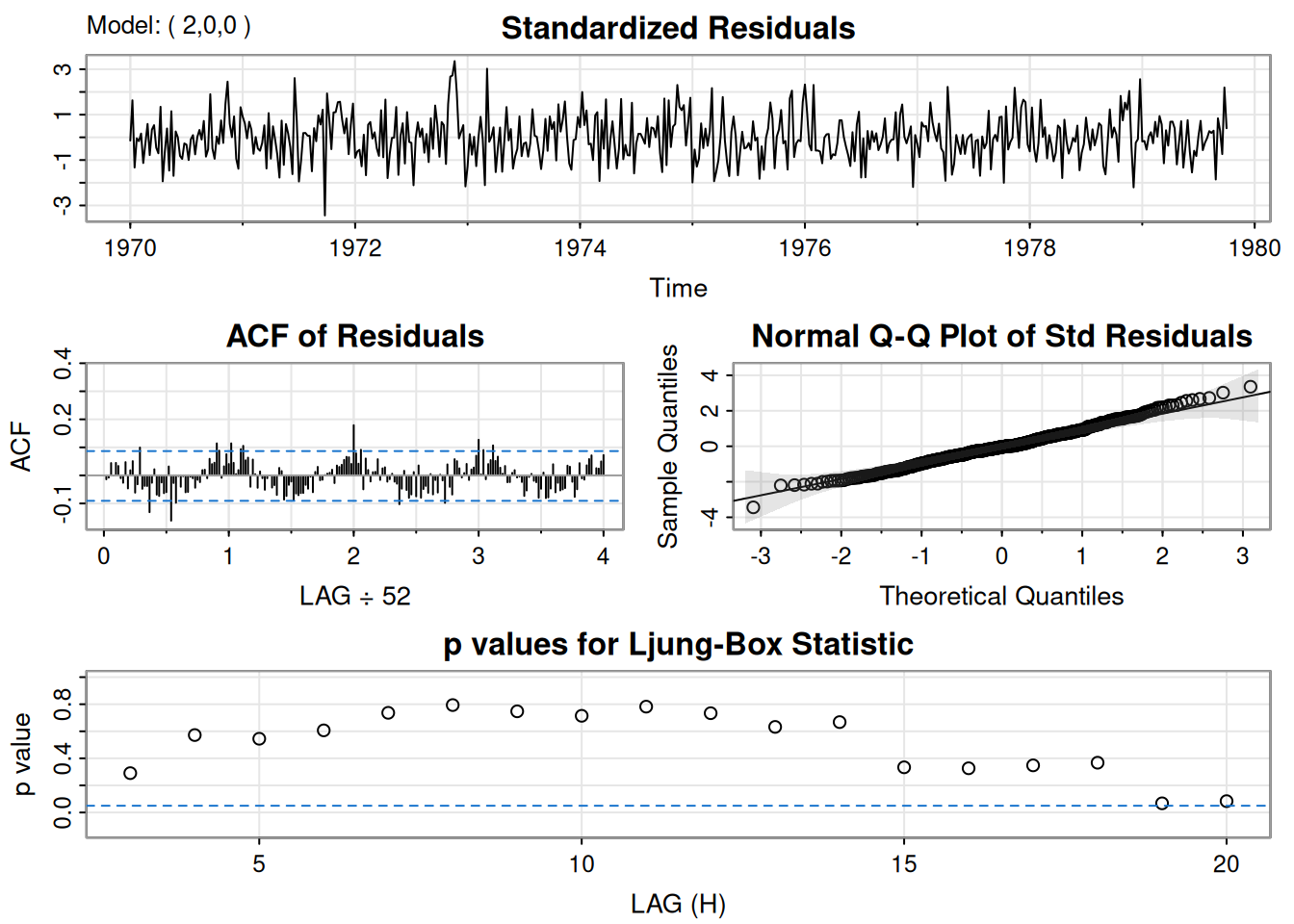
Salida parcial:
Coefficients:
    ar1    ar2    intercept   trend   temp   temp2   part
 s.e. 0.0436 0.0400 1.8072 0.4226 0.0495 0.0020 0.0272
sigma^2 estimated as 26.01: loglikelihood = -1549.04, aic = 3114.07
Los residuales muestran comportamiento de ruido blanco.
Modelo inicial:
\[ R_t=\beta_0+\beta_1 S_{t-6}+\beta_2 D_{t-6}+\beta_3 D_{t-6}S_{t-6}+w_t, \]
donde \(R_t\) es reclutamiento, \(S_t\) es SOI y \(D_t\) es variable dummy (\(0\) si \(S_t<0\), \(1\) en otro caso). ACF y PACF de los residuales sugieren un AR(2).
dummy = ifelse(soi<0, 0, 1)
fish = ts.intersect(rec, soiL6=stats::lag(soi,-6), dL6=stats::lag(dummy,-6), dframe=TRUE)
summary(fit <- lm(rec ~ soiL6*dL6, data=fish, na.action=NULL))
Call:
lm(formula = rec ~ soiL6 * dL6, data = fish, na.action = NULL)

Residuals:
    Min      1Q  Median      3Q     Max
-63.291 -15.821   2.224  15.791  61.788

Coefficients:
            Estimate Std. Error t value Pr(>|t|)
(Intercept)   74.479      2.865  25.998  < 2e-16 ***
soiL6        -15.358      7.401  -2.075   0.0386 *
dL6           -1.139      3.711  -0.307   0.7590
soiL6:dL6    -51.244      9.523  -5.381  1.2e-07 ***
---
Signif. codes:  0 '***' 0.001 '**' 0.01 '*' 0.05 '.' 0.1 ' ' 1

Residual standard error: 21.84 on 443 degrees of freedom
Multiple R-squared:  0.4024,    Adjusted R-squared:  0.3984
F-statistic: 99.43 on 3 and 443 DF, p-value: < 2.2e-16attach(fish)The following object is masked from package:astsa:
recplot(resid(fit))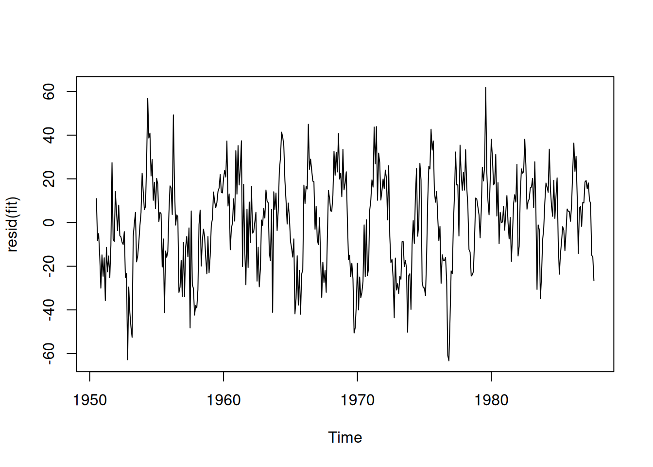
acf2(resid(fit)) # sugiere AR(2)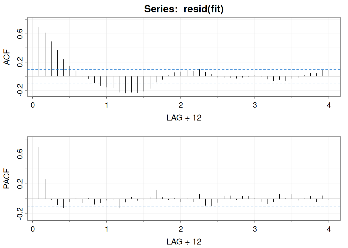
     [,1] [,2]  [,3]  [,4]  [,5]  [,6] [,7]  [,8]  [,9] [,10] [,11] [,12] [,13]
ACF  0.69 0.62  0.49  0.37  0.24  0.15 0.08  0.00 -0.03 -0.10 -0.13 -0.16 -0.17
PACF 0.69 0.26 -0.01 -0.08 -0.12 -0.04 0.01 -0.05  0.01 -0.07 -0.05 -0.02 -0.01
     [,14] [,15] [,16] [,17] [,18] [,19] [,20] [,21] [,22] [,23] [,24] [,25]
ACF  -0.23 -0.24 -0.23 -0.23 -0.22 -0.17 -0.09 -0.05  0.01  0.05  0.06  0.09
PACF -0.12 -0.04  0.02 -0.02  0.00  0.03  0.12  0.02 -0.01  0.01 -0.04  0.00
     [,26] [,27] [,28] [,29] [,30] [,31] [,32] [,33] [,34] [,35] [,36] [,37]
ACF   0.07  0.10  0.06  0.02 -0.02 -0.02 -0.02 -0.03 -0.02  0.00  0.01 -0.01
PACF -0.04  0.06 -0.09 -0.10 -0.05  0.04  0.04 -0.01  0.03  0.04  0.01 -0.04
     [,38] [,39] [,40] [,41] [,42] [,43] [,44] [,45] [,46] [,47] [,48]
ACF  -0.04 -0.07 -0.05 -0.06 -0.03 -0.02  0.01  0.04  0.04  0.08  0.08
PACF -0.07 -0.04  0.06  0.01  0.06 -0.02  0.00  0.03 -0.04  0.04 -0.01
intract = soiL6*dL6
sarima(rec,2,0,0, xreg = cbind(soiL6, dL6, intract))initial value 3.080982
iter 2 value 2.921817
iter 3 value 2.671207
iter 4 value 2.554389
iter 5 value 2.404164
iter 6 value 2.365228
iter 7 value 2.256092
iter 8 value 2.240552
iter 9 value 2.238427
iter 10 value 2.232931
iter 11 value 2.232826
iter 12 value 2.232765
iter 13 value 2.232755
iter 14 value 2.232750
iter 15 value 2.232750
iter 16 value 2.232749
iter 17 value 2.232749
iter 17 value 2.232749
iter 17 value 2.232749
final value 2.232749
converged
initial value 2.234466
iter 2 value 2.234463
iter 3 value 2.234460
iter 4 value 2.234460
iter 5 value 2.234459
iter 6 value 2.234459
iter 7 value 2.234458
iter 8 value 2.234456
iter 9 value 2.234455
iter 10 value 2.234454
iter 11 value 2.234453
iter 11 value 2.234453
iter 11 value 2.234453
final value 2.234453
converged
<><><><><><><><><><><><><><>
Coefficients:
Estimate SE t.value p.value
ar1 1.3624 0.0440 30.9303 0.0000
ar2 -0.4703 0.0444 -10.5902 0.0000
intercept 64.8028 4.1121 15.7590 0.0000
soiL6 8.6671 2.2205 3.9033 0.0001
dL6 -2.5945 0.9535 -2.7209 0.0068
intract -10.3092 2.8311 -3.6415 0.0003
sigma^2 estimated as 86.78315 on 441 degrees of freedom
AIC = 7.338104 AICc = 7.338531 BIC = 7.40235
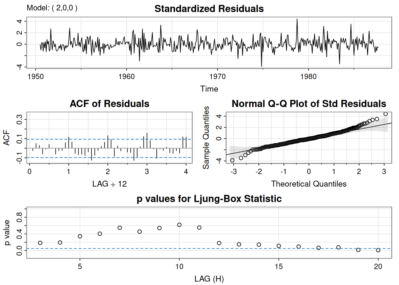
Se presentan las extensiones de los modelos ARIMA para capturar patrones estacionales, conocidos como modelos SARMA y SARIMA. Estos modelos consideran dependencias en rezagos múltiplos de un período estacional \(s\), común en datos económicos, climáticos y biológicos. Se detallan condiciones de causalidad e invertibilidad, ejemplos simulados y aplicaciones reales con datos de pasajeros aéreos internacionales.
Un modelo ARMA puramente estacional se expresa como:
\[ \Phi_{P}\left(B^{s}\right) x_{t}=\Theta_{Q}\left(B^{s}\right) w_{t}, \]
con operadores estacionales:
\[ \Phi_{P}\left(B^{s}\right)=1-\Phi_{1} B^{s}-\Phi_{2} B^{2s}-\cdots-\Phi_{P} B^{Ps}, \]
\[ \Theta_{Q}\left(B^{s}\right)=1+\Theta_{1} B^{s}+\Theta_{2} B^{2s}+\cdots+\Theta_{Q} B^{Qs}. \]
El proceso es causal si las raíces de \(\Phi_{P}(z^s)\) están fuera del círculo unitario e invertible si las raíces de \(\Theta_{Q}(z^s)\) están fuera de dicho círculo.
Modelo:
\[ (1-\Phi B^{12})x_t=w_t, \quad x_t=\Phi x_{t-12}+w_t. \]
Con \(\Phi=.9\) se simulan tres años de datos:
set.seed(666)
phi = c(rep(0,11),.9)
sAR = arima.sim(list(order=c(12,0,0), ar=phi), n=37)
sAR = ts(sAR, freq=12)
layout(matrix(c(1,1,2, 1,1,3), nc=2))
par(mar=c(3,3,2,1), mgp=c(1.6,.6,0))
plot(sAR, axes=FALSE, main='seasonal AR(1)', xlab="year", type='c')
Months = c("J","F","M","А","M","J","J","А","S","О","N","D")
points(sAR, pch=Months, cex=1.25, font=4, col=1:4)
axis(1, 1:4); abline(v=1:4, lty=2, col=gray(.7))
axis(2); box()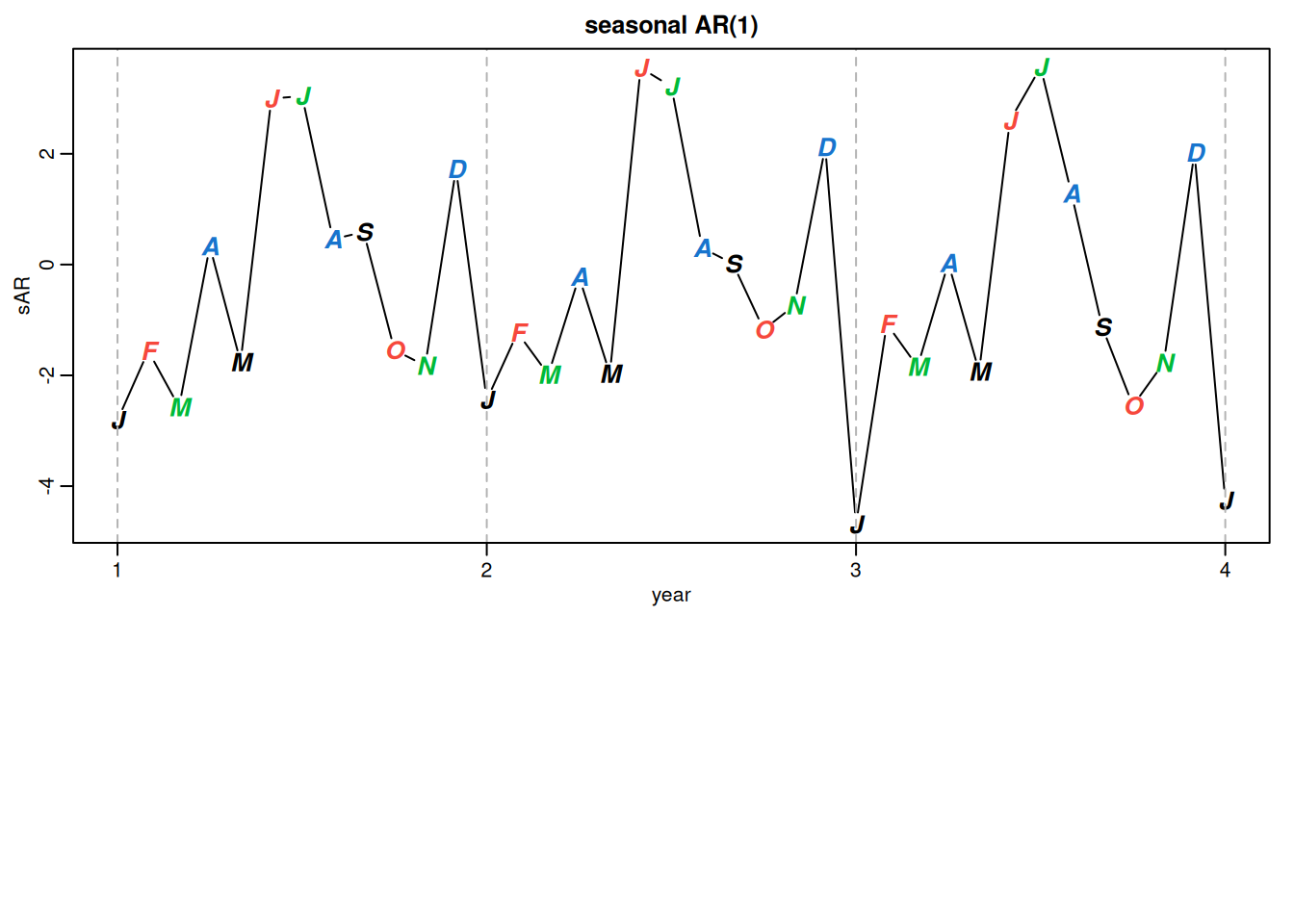
Cálculo de ACF y PACF teóricos:
ACF = ARMAacf(ar=phi, ma=0, 100)
PACF = ARMAacf(ar=phi, ma=0, 100, pacf=TRUE)
plot(ACF,type="h", xlab="LAG", ylim=c(-.1,1)); abline(h=0)
plot(PACF, type="h", xlab="LAG", ylim=c(-.1,1)); abline(h=0)
Autocovarianzas para MA(1) y AR(1) estacionales:
\[ \gamma(0)=(1+\Theta^2)\sigma^2,\quad \gamma(\pm 12)=\Theta\sigma^2,\quad \gamma(h)=0 \ \text{otros}. \]
\[ \gamma(0)=\frac{\sigma^2}{1-\Phi^2},\quad \gamma(\pm 12k)=\frac{\sigma^2\Phi^k}{1-\Phi^2},\quad \gamma(h)=0 \ \text{otros}. \]
Modelo general:
\[ \Phi_P(B^s)\phi(B)x_t=\Theta_Q(B^s)\theta(B)w_t. \]
Las propiedades de ACF y PACF de los modelos SARMA puros se resumen en la siguiente tabla, como extensión de los casos no estacionales:
Comportamiento de la ACF y PACF para modelos SARMA puros
| AR(P)ₛ | MA(Q)ₛ | ARMA(P,Q)ₛ | |
|---|---|---|---|
| ACF* | Se atenúa en rezagos ks, | Se corta después del rezago Qs | Se atenúa en rezagos ks |
| k = 1, 2, … | |||
| PACF* | Se corta después del rezago Ps | Se atenúa en rezagos ks, | Se atenúa en rezagos ks |
| k = 1, 2, … |
*Los valores en rezagos no estacionales \(h \neq ks\), para \(k = 1, 2, \ldots\), son cero.
Modelo \(\operatorname{ARMA}(0,1)\times(1,0)_{12}\):
\[ x_t=\Phi x_{t-12}+w_t+\theta w_{t-1}. \]
Autocovarianza en \(h=0\):
\[ \gamma(0)=\frac{1+\theta^2}{1-\Phi^2}\sigma_w^2. \]
Autocorrelaciones:
\[ \rho(12h)=\Phi^h,\quad \rho(12h\pm 1)=\frac{\theta}{1+\theta^2}\Phi^h,\quad \rho(h)=0 \ \text{otros}. \]
Código en R para ACF y PACF con \(\Phi=.8\), \(\theta=-.5\):
phi = c(rep(0,11),.8)
ACF = ARMAacf(ar=phi, ma=-.5, 50)[-1]
PACF = ARMAacf(ar=phi, ma=-.5, 50, pacf=TRUE)
par(mfrow=c(1,2))
plot(ACF, type="h", xlab="LAG", ylim=c(-.4,.8)); abline(h=0)
plot(PACF, type="h", xlab="LAG", ylim=c(-.4,.8)); abline(h=0)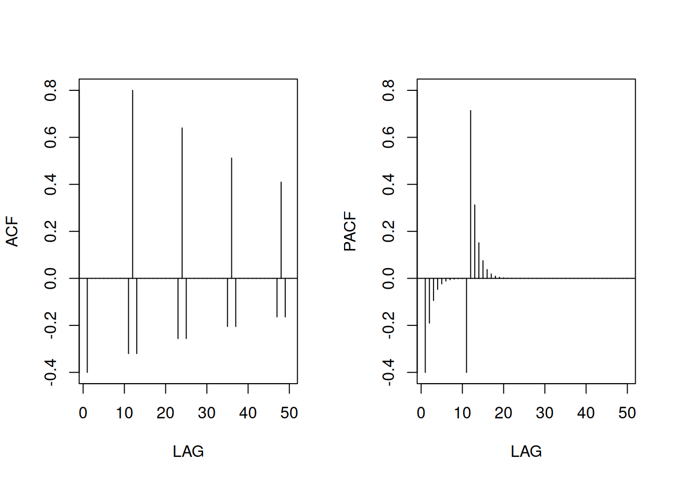
Si los datos presentan persistencia estacional, se puede aplicar diferenciación:
\[ \nabla_s^D x_t=(1-B^s)^D x_t. \]
Modelo general SARIMA:
\[ \Phi_P(B^s)\phi(B)\nabla_s^D\nabla^d x_t=\delta+\Theta_Q(B^s)\theta(B)w_t. \]
Modelo \(\operatorname{ARIMA}(0,1,1)\times(0,1,1)_{12}\):
\[ (1-B^{12})(1-B)x_t=(1+\Theta B^{12})(1+\theta B)w_t. \]
Forma en ecuaciones de diferencias:
\[ x_t=x_{t-1}+x_{t-12}-x_{t-13}+w_t+\theta w_{t-1}+\Theta w_{t-12}+\Theta\theta w_{t-13}. \]
Datos mensuales 1949–1960 (AirPassengers). Transformaciones:
x = AirPassengers
lx = log(x); dlx = diff(lx); ddlx = diff(dlx, 12)
plot.ts(cbind(x,lx,dlx,ddlx), main="")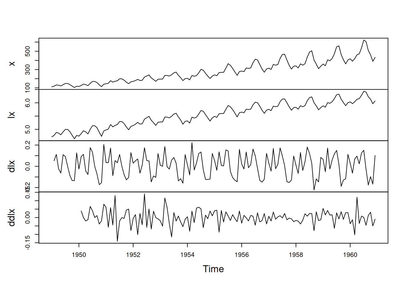
par(mfrow=c(2,1))
monthplot(dlx); monthplot(ddlx)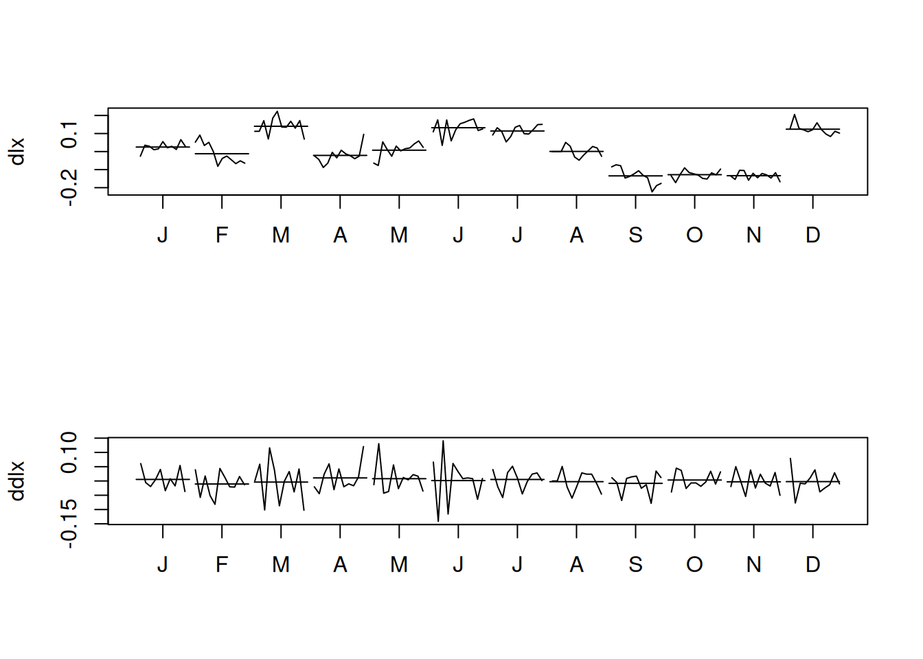
ACF y PACF de \(\nabla_{12}\nabla \log x_t\):
acf2(ddlx, 50)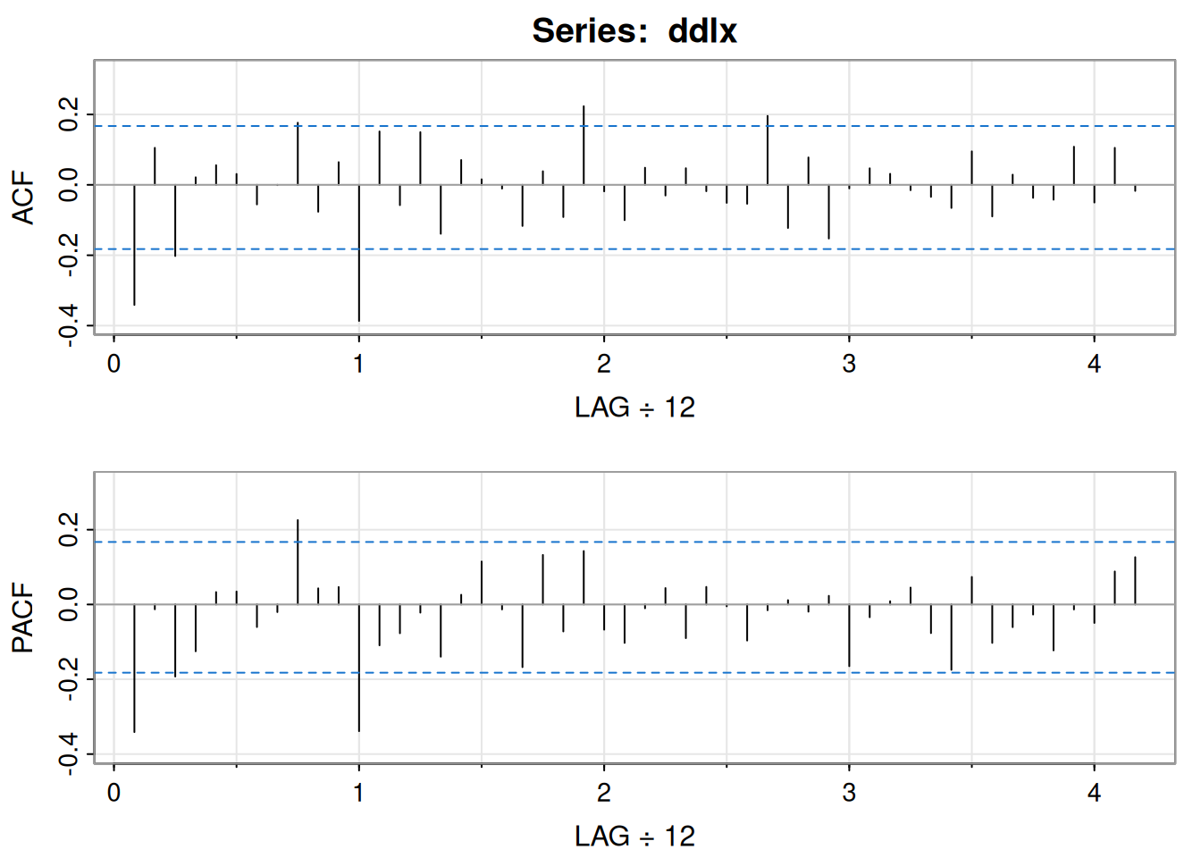
      [,1]  [,2]  [,3]  [,4] [,5] [,6]  [,7]  [,8] [,9] [,10] [,11] [,12] [,13]
ACF  -0.34  0.11 -0.20  0.02 0.06 0.03 -0.06  0.00 0.18 -0.08  0.06 -0.39  0.15
PACF -0.34 -0.01 -0.19 -0.13 0.03 0.03 -0.06 -0.02 0.23  0.04  0.05 -0.34 -0.11
     [,14] [,15] [,16] [,17] [,18] [,19] [,20] [,21] [,22] [,23] [,24] [,25]
ACF  -0.06  0.15 -0.14  0.07  0.02 -0.01 -0.12  0.04 -0.09  0.22 -0.02  -0.1
PACF -0.08 -0.02 -0.14  0.03  0.11 -0.01 -0.17  0.13 -0.07  0.14 -0.07  -0.1
     [,26] [,27] [,28] [,29] [,30] [,31] [,32] [,33] [,34] [,35] [,36] [,37]
ACF   0.05 -0.03  0.05 -0.02 -0.05 -0.05  0.20 -0.12  0.08 -0.15 -0.01  0.05
PACF -0.01  0.04 -0.09  0.05  0.00 -0.10 -0.02  0.01 -0.02  0.02 -0.16 -0.03
     [,38] [,39] [,40] [,41] [,42] [,43] [,44] [,45] [,46] [,47] [,48] [,49]
ACF   0.03 -0.02 -0.03 -0.07  0.10 -0.09  0.03 -0.04 -0.04  0.11 -0.05  0.11
PACF  0.01  0.05 -0.08 -0.17  0.07 -0.10 -0.06 -0.03 -0.12 -0.01 -0.05  0.09
     [,50]
ACF  -0.02
PACF  0.13
Se propone un modelo ARIMA(1,1,1)\(\times\)(0,1,1)\(_{12}\):
sarima(lx, 1,1,1, 0,1,1,12)initial value -3.085211
iter 2 value -3.225399
iter 3 value -3.276697
iter 4 value -3.276902
iter 5 value -3.282134
iter 6 value -3.282524
iter 7 value -3.282990
iter 8 value -3.286319
iter 9 value -3.286413
iter 10 value -3.288141
iter 11 value -3.288262
iter 12 value -3.288394
iter 13 value -3.288768
iter 14 value -3.288969
iter 15 value -3.289089
iter 16 value -3.289094
iter 17 value -3.289100
iter 17 value -3.289100
iter 17 value -3.289100
final value -3.289100
converged
initial value -3.288388
iter 2 value -3.288459
iter 3 value -3.288530
iter 4 value -3.288649
iter 5 value -3.288753
iter 6 value -3.288781
iter 7 value -3.288784
iter 7 value -3.288784
iter 7 value -3.288784
final value -3.288784
converged
<><><><><><><><><><><><><><>
Coefficients:
Estimate SE t.value p.value
ar1 0.1960 0.2475 0.7921 0.4298
ma1 -0.5784 0.2132 -2.7127 0.0076
sma1 -0.5643 0.0747 -7.5544 0.0000
sigma^2 estimated as 0.001341097 on 128 degrees of freedom
AIC = -3.678622 AICc = -3.677179 BIC = -3.59083
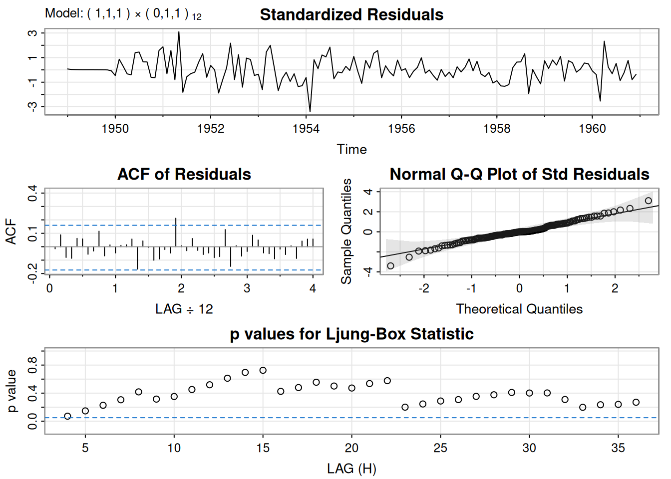
Coeficientes estimados:
ar1   ma1   sma1
0.1960 -0.5784 -0.5643
El parámetro AR no es significativo, se prueban simplificaciones:
sarima(lx, 0,1,1, 0,1,1,12)initial value -3.086228
iter 2 value -3.267980
iter 3 value -3.279950
iter 4 value -3.285996
iter 5 value -3.289332
iter 6 value -3.289665
iter 7 value -3.289672
iter 8 value -3.289676
iter 8 value -3.289676
iter 8 value -3.289676
final value -3.289676
converged
initial value -3.286464
iter 2 value -3.286855
iter 3 value -3.286872
iter 4 value -3.286874
iter 4 value -3.286874
iter 4 value -3.286874
final value -3.286874
converged
<><><><><><><><><><><><><><>
Coefficients:
Estimate SE t.value p.value
ma1 -0.4018 0.0896 -4.4825 0
sma1 -0.5569 0.0731 -7.6190 0
sigma^2 estimated as 0.001348035 on 129 degrees of freedom
AIC = -3.690069 AICc = -3.689354 BIC = -3.624225

sarima(lx, 1,1,0, 0,1,1,12)initial value -3.085211
iter 2 value -3.259459
iter 3 value -3.262637
iter 4 value -3.275171
iter 5 value -3.277007
iter 6 value -3.277205
iter 7 value -3.277208
iter 8 value -3.277209
iter 8 value -3.277209
iter 8 value -3.277209
final value -3.277209
converged
initial value -3.279535
iter 2 value -3.279580
iter 3 value -3.279586
iter 3 value -3.279586
iter 3 value -3.279586
final value -3.279586
converged
<><><><><><><><><><><><><><>
Coefficients:
Estimate SE t.value p.value
ar1 -0.3395 0.0822 -4.1295 1e-04
sma1 -0.5619 0.0748 -7.5109 0e+00
sigma^2 estimated as 0.00136738 on 129 degrees of freedom
AIC = -3.675493 AICc = -3.674777 BIC = -3.609649

Todos los criterios de información favorecen el modelo ARIMA(0,1,1)\(\times\)(0,1,1)\(_{12}\).
Pronóstico a 12 meses:
sarima.for(lx, 12, 0,1,1, 0,1,1,12)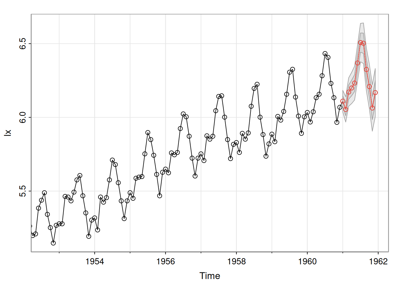
$pred
          Jan      Feb      Mar      Apr      May      Jun      Jul      Aug
1961 6.110186 6.053775 6.171715 6.199300 6.232556 6.368779 6.507294 6.502906
          Sep      Oct      Nov      Dec
1961 6.324698 6.209008 6.063487 6.168025

$se
            Jan        Feb        Mar        Apr        May        Jun
1961 0.03671562 0.04278291 0.04809072 0.05286830 0.05724856 0.06131670
            Jul        Aug        Sep        Oct        Nov        Dec
1961 0.06513124 0.06873441 0.07215787 0.07542612 0.07855851 0.08157070