5.1.1 Modelo base y problema de sobrediferenciación
Sea el proceso AR(1) causal (ruido gaussiano): \[
x_t=\phi x_{t-1}+w_t.
\]
Aplicando \((1-B)\) a ambos lados: \[
\nabla x_t=\phi \nabla x_{t-1}+\nabla w_t,\quad
y_t=\phi y_{t-1}+w_t-w_{t-1},
\] donde \(y_t=\nabla x_t\). Así, \(y_t\) es un ARMA\((1,1)\) no invertible: diferenciar puede introducir correlación espuria y problemas de invertibilidad.
Bajo una caminata aleatoria \(x_t=x_{t-1}+w_t\) con \(x_0=0\) y \(\mu_x=0\), el estimador LS es \[
\hat{\phi}=\frac{\sum_{t=1}^{n} x_t x_{t-1}}{\sum_{t=1}^{n} x_{t-1}^2}
=1+\frac{\frac{1}{n}\sum_{t=1}^{n} w_t x_{t-1}}{\frac{1}{n}\sum_{t=1}^{n} x_{t-1}^2}.
\] Por tanto, \[
\hat{\phi}-1=\frac{\frac{1}{n\sigma_w^2}\sum_{t=1}^{n} w_t x_{t-1}}
{\frac{1}{n\sigma_w^2}\sum_{t=1}^{n} x_{t-1}^2}.
\]
Dado \(x_t=x_{t-1}+w_t\), se tiene \(x_t^2=x_{t-1}^2+2x_{t-1}w_t+w_t^2\), luego \[
x_{t-1}w_t=\tfrac{1}{2}\left(x_t^2-x_{t-1}^2-w_t^2\right),
\] y al sumar, \[
\frac{1}{n\sigma_w^2}\sum_{t=1}^{n}x_{t-1}w_t
=\frac{1}{2}\left(\frac{x_n^2}{n\sigma_w^2}-\frac{\sum_{t=1}^{n}w_t^2}{n\sigma_w^2}\right).
\] Como \(x_n=\sum_{1}^{n}w_t\sim N(0,n\sigma_w^2)\), entonces \(\chi_1^2=\frac{x_n^2}{n\sigma_w^2}\) y \(\frac{1}{n}\sum_{1}^{n}w_t^2\to_p \sigma_w^2\). En consecuencia, \[
\frac{1}{n\sigma_w^2}\sum_{t=1}^{n}x_{t-1}w_t \xrightarrow{d} \tfrac{1}{2}\left(\chi_1^2-1\right).
\]
5.1.3 Movimiento browniano estándar
Un proceso continuo \({W(t);t\ge 0}\) es browniano estándar si:
\(W(0)=0\);
incrementos independientes en puntos \(0\le t_1<\cdots<t_n\);
\(W(t+\Delta t)-W(t)\sim N(0,\Delta t)\) para \(\Delta t>0\), con trayectorias casi seguramente continuas.
5.1.3.1 Teorema central funcional
Si \(\xi_1,\ldots,\xi_n\) iid con media 0 y varianza 1, para \(0\le t\le 1\): \[
S_n(t)=\frac{1}{\sqrt{n}}\sum_{j=1}^{[[ nt]]}\xi_j \xrightarrow{d} W(t).
\] Bajo \(H_0\), \(x_s=w_1+\cdots+w_s\sim N(0,s\sigma_w^2)\) y \(\frac{x_s}{\sigma_w\sqrt{n}}\xrightarrow{d}W(s)\). Por tanto, \[
\sum_{t=1}^{n}\left(\frac{x_{t-1}}{\sigma_w\sqrt{n}}\right)^2\frac{1}{n}
\xrightarrow{d}\int_{0}^{1}W^2(t),dt.
\]
5.1.4 Estadístico DF y su límite
Ajustando el factor \(n^{-1}\) del denominador de la expresión de \(\hat \phi-1\):
\[
n(\hat{\phi}-1)=
\frac{\frac{1}{n\sigma_w^2}\sum_{t=1}^{n} w_t x_{t-1}}
{\frac{1}{n^{2}\sigma_w^2}\sum_{t=1}^{n} x_{t-1}^{2}}
\xrightarrow{d}\frac{\tfrac{1}{2}\left(\chi_1^2-1\right)}
{\int_{0}^{1}W^2(t),dt}.
\] Este es el estadístico de Dickey–Fuller (DF). Su distribución no tiene forma cerrada; los cuantiles se obtienen por aproximación numérica o simulación.
5.1.5 Extensiones DF/ADF/PP
Reescribiendo \(x_t=\phi x_{t-1}+w_t\) como \(\nabla x_t=\gamma x_{t-1}+w_t\) con \(\gamma=\phi-1\), se prueba \(H_0:\gamma=0\) por regresión de \(\nabla x_t\) sobre \(x_{t-1}\). Para AR(\(p\)): \[
\nabla x_t=\gamma x_{t-1}+\sum_{j=1}^{p-1}\psi_j \nabla x_{t-j}+w_t,
\] donde \(\gamma=\sum_{j=1}^{p}\phi_j-1\) y \(\psi_j=-\sum_{i=j}^{p}\phi_i\) para \(j=2,\ldots,p\). El ADF contrasta \(H_0:\gamma=0\) vía \(t_\gamma=\hat\gamma/\operatorname{se}(\hat\gamma)\) en la regresión sobre \(x_{t-1},\nabla x_{t-1},\ldots,\nabla x_{t-p+1}\). Para ARMA\((p,q)\) se usa ADF con \(p\) grande o el test de Phillips–Perron (PP), que trata de forma distinta la correlación serial y heterocedasticidad en los errores.
5.1.5.1 Ejemplo: Pruebas de raíz unitaria en la serie de varves glaciares
A continuación se usan pruebas DF, ADF y PP sobre el logaritmo de la serie de varves glaciares (cada prueba incluye constante y tendencia lineal). En ADF, el número de retardos AR \(k\) por defecto es \([[(n-1)^{1/3}]]\); en PP, \(k=[[ 0.04n^{1/4}]]\).
library(tidyverse)
── Attaching core tidyverse packages ──────────────────────── tidyverse 2.0.0 ──
✔ dplyr     1.1.4     ✔ readr     2.1.5
✔ forcats   1.0.0     ✔ stringr   1.5.2
✔ ggplot2   4.0.0     ✔ tibble    3.3.0
✔ lubridate 1.9.4     ✔ tidyr     1.3.1
✔ purrr     1.1.0
── Conflicts ────────────────────────────────────────── tidyverse_conflicts() ──
✖ dplyr::filter() masks stats::filter()
✖ dplyr::lag()    masks stats::lag()
ℹ Use the conflicted package (<http://conflicted.r-lib.org/>) to force all conflicts to become errors
library(astsa)library(tseries)
Registered S3 method overwritten by 'quantmod':
  method            from
  as.zoo.data.frame zoo
adf.test(log(varve), k =0) # DF
Warning in adf.test(log(varve), k = 0): p-value smaller than printed p-value
    Augmented Dickey-Fuller Test

data:  log(varve)
Dickey-Fuller = -12.857, Lag order = 0, p-value = 0.01
alternative hypothesis: stationary
adf.test(log(varve)) # ADF (k por defecto)
    Augmented Dickey-Fuller Test

data:  log(varve)
Dickey-Fuller = -3.5166, Lag order = 8, p-value = 0.04071
alternative hypothesis: stationary
pp.test(log(varve)) # PP
Warning in pp.test(log(varve)): p-value smaller than printed p-value
    Phillips-Perron Unit Root Test

data:  log(varve)
Dickey-Fuller Z(alpha) = -304.54, Truncation lag parameter = 6, p-value
= 0.01
alternative hypothesis: stationary
5.2 Modelos GARCH
5.2.1 Modelado de volatilidad: retornos y motivación
Si \(x_t\) es el valor del activo en \(t\), el retorno relativo es \[
r_t=\frac{x_t-x_{t-1}}{x_{t-1}}.
\] Como \(x_t=(1+r_t)x_{t-1}\), si el cambio porcentual es pequeño: \[
\nabla\log(x_t)\approx r_t.
\] Usaremos indistintamente \(r_t\equiv \nabla\log(x_t)\) o \((x_t-x_{t-1})/x_{t-1}\).
5.2.2 Modelo ARCH(1): definición y propiedades
5.2.2.1 Especificación básica
\[
\begin{aligned}
r_t&=\sigma_t\epsilon_t, \\
\sigma_t^2&=\alpha_0+\alpha_1 r_{t-1}^2,
\end{aligned}
\] con \(\epsilon_t\sim \text{iid }N(0,1)\) y \(\alpha_0,\alpha_1\ge 0\).
La distribución condicional: \[
r_t\mid r_{t-1}\sim N\left(0,\ \alpha_0+\alpha_1 r_{t-1}^2\right).
\]
5.2.2.2 Representación para \(r_t^2\)
A partir de la definición del modelo ARCH: \[
\begin{aligned}
r_t^2 &= \sigma_t^2 \, \epsilon_t^2, \\
\alpha_0 + \alpha_1 r_{t-1}^2 &= \sigma_t^2,
\end{aligned}
\] y restando ambas ecuaciones se obtiene:
\[
r_t^2 - \left( \alpha_0 + \alpha_1 r_{t-1}^2 \right) = \sigma_t^2 (\epsilon_t^2 - 1),
\] de donde se obtiene:
\[
r_t^2=\alpha_0+\alpha_1 r_{t-1}^2+v_t,\quad v_t=\sigma_t^2(\epsilon_t^2-1),
\] donde \(\epsilon_t^2-1\) es \(\chi_1^2\) desplazada o centrada en 0.
Propiedades
Sea \(\mathcal{R}_s=\{r_s,r_{s-1},\ldots\}\). Entonces \[
\mathrm{E}(r_t)=\mathrm{E}[{\mathrm{E}(r_t\mid \mathcal{R}_{t-1})}]
=\mathrm{E}[{\mathrm{E}(r_t\mid r_{t-1})}]=0,
\] por lo tanto es una diferencia martingala y para \(h>0\), \[
\operatorname{cov}(r_{t+h},r_t)=\mathrm{E}{r_t\mathrm{E}(r_{t+h}\mid\mathcal{R}_{t+h-1})}=0.
\]
Si \(0\le \alpha_1<1\) y \(\operatorname{var}(v_t)\) es finita y constante entonces \(r_t^2\) es AR(1) causal (estacionario), por lo que \[
\mathrm{E}(r_t^2)=\operatorname{var}(r_t)=\frac{\alpha_0}{1-\alpha_1},
\] y \[
\mathrm{E}(r_t^4)=\frac{3\alpha_0^2}{(1-\alpha_1)^2}\cdot \frac{1-\alpha_1^2}{1-3\alpha_1^2},\quad (3\alpha_1^2<1).
\] La curtosis es \[
\kappa=\frac{\mathrm{E}(r_t^4)}{[\mathrm{E}(r_t^2)]^2}=3\frac{1-\alpha_1^2}{1-3\alpha_1^2}\ge 3,
\] lo que indica colas pesadas (leptocurtosis). Si \(3\alpha_1^2<1\), \(\rho_{r^2}(h)=\alpha_1^h\ge 0\).
5.2.3 Estimación por verosimilitud condicional
La verosimilitud condicional de \(r_2,\ldots,r_n\) dado \(r_1\) es \[
L(\alpha_0,\alpha_1\mid r_1)=\prod_{t=2}^n f_{\alpha_0,\alpha_1}(r_t\mid r_{t-1}),
\] y el criterio a minimizar es \[
l(\alpha_0,\alpha_1)=\tfrac{1}{2}\sum_{t=2}^n \ln(\alpha_0+\alpha_1 r_{t-1}^2)
+\tfrac{1}{2}\sum_{t=2}^n \frac{r_t^2}{\alpha_0+\alpha_1 r_{t-1}^2}.
\] El MLE solamente se obtiene por métodos numéricos. Para esto se necesita el gradiente: \[
\binom{\partial l/\partial \alpha_0}{\partial l/\partial \alpha_1}
=\sum_{t=2}^n \binom{1}{r_{t-1}^2}
\frac{\alpha_0+\alpha_1 r_{t-1}^2-r_t^2}{2(\alpha_0+\alpha_1 r_{t-1}^2)^2}.
\]
Nota: la logverosimilitud para este tipo de modelo tiende a ser muy plana.
También es posible combinar un modelo de regresión con errores ARCH:
\[
x_t=\beta^t z_t+y_t
\] donde \(y_t\) es ARCH. En particular un AR(1) podría tener errores ARCH:
\[
\sigma_t^2=\alpha_0+\alpha_1 r_{t-1}^2+\beta_1 \sigma_{t-1}^2,
\] y si \(\alpha_1+\beta_1<1\), \[
r_t^2=\alpha_0+(\alpha_1+\beta_1) r_{t-1}^2+v_t-\beta_1 v_{t-1}.
\] donde \(v_t\) se definió anteriormente.
La estimación de máxima verosimilitud condicional de los parámetros del modelo GARCH\((p,q)\) es similar al caso ARCH\((p)\), en el cual la verosimilitud condicional es el producto de densidades \(\mathrm{N}(0, \sigma_t^2)\) con \(\sigma_t^2\) dado por la ecuación anterior, y donde la condición se establece sobre las primeras \(\max(p,q)\) observaciones, con \(\sigma_1^2 = \cdots = \sigma_q^2 = 0\). Una vez que se obtienen las estimaciones de los parámetros, el modelo puede utilizarse para obtener pronósticos de volatilidad de un paso adelante, denotados como \(\hat{\sigma}_{t+1}^2\), dados por
En series financieras (y otras), la varianza condicional puede cambiar en el tiempo: periodos de alta volatilidad tienden a agruparse. Los modelos ARCH/GARCH modelan esa heterocedasticidad condicional.
Sea \({\varepsilon_t}\) la secuencia de residuos (por ejemplo, de un modelo para la media). Decimos que hay efecto ARCH de orden \(q\) si la varianza condicional en \(t\) depende de los cuadrados de los últimos \(q\) residuos: \[
\operatorname{Var}(\varepsilon_t\mid \mathcal F_{t-1}) = \alpha_0 + \alpha_1\varepsilon_{t-1}^2 + \cdots + \alpha_q\varepsilon_{t-q}^2,
\quad \alpha_0>0, \alpha_j\ge 0.
\]
La prueba LM ARCH (Engle) contrasta:
\(H_0\): no hay efecto ARCH (varianza condicional constante; \(\alpha_1=\cdots=\alpha_q=0\)).
\(H_1\): sí hay efecto ARCH de algún orden (\(\exists j:\alpha_j\ne 0\)).
Regresión auxiliar y estadístico
La prueba se implementa ajustando la regresión sobre los residuos al cuadrado: \[
\hat{\varepsilon}_t^2 =\alpha_0+\alpha_1\hat{\varepsilon}_{t-1}^2+\cdots+\alpha_q \hat{\varepsilon}_{t-q}^2+u_t.
\]
Sea \(R^2\) el coeficiente de determinación de esta regresión y \(n\) el número de observaciones usadas. El estadístico LM es: \[
\text{LM}=nR^2 \overset{H_0}{\approx}\chi^2_q.
\]
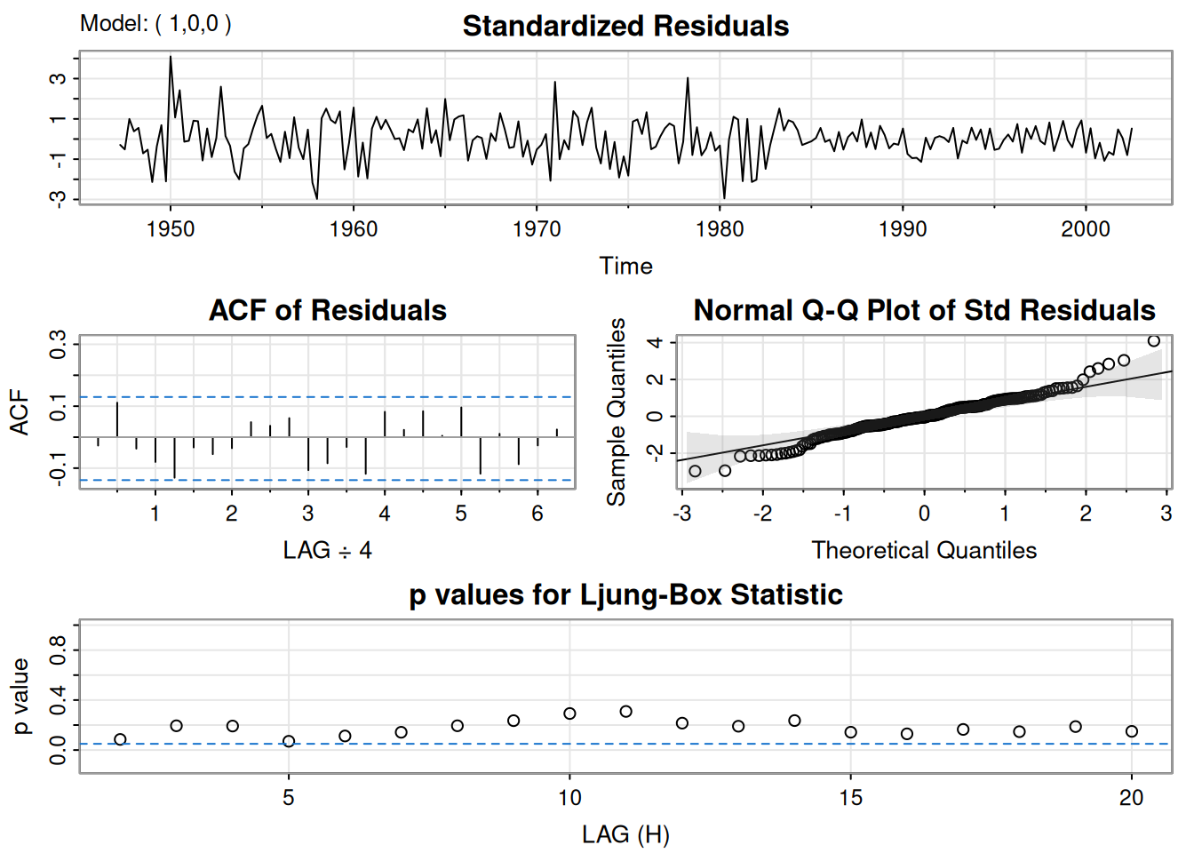
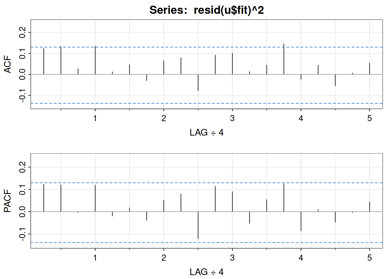
5.2.5.1 Ejemplo: Análisis ARCH en U.S. GNP
La ACF/PACF de los cuadrados de los residuales del AR(1) sugiere dependencia débil.
u =sarima(diff(log(gnp)), 1, 0, 0)
initial  value -4.589567
iter   2 value -4.654150
iter   3 value -4.654150
iter   4 value -4.654151
iter   4 value -4.654151
iter   4 value -4.654151
final  value -4.654151
converged
initial  value -4.655919
iter   2 value -4.655921
iter   3 value -4.655922
iter   4 value -4.655922
iter   5 value -4.655922
iter   5 value -4.655922
iter   5 value -4.655922
final  value -4.655922
converged
<><><><><><><><><><><><><><>

Coefficients:
      Estimate     SE t.value p.value
ar1     0.3467 0.0627  5.5255       0
xmean   0.0083 0.0010  8.5398       0

sigma^2 estimated as 9.029569e-05 on 220 degrees of freedom

AIC = -6.44694  AICc = -6.446693  BIC = -6.400958
NOTE: Packages 'fBasics', 'timeDate', and 'timeSeries' are no longer
attached to the search() path when 'fGarch' is attached.

If needed attach them yourself in your R script by e.g.,
        require("timeSeries")
Series Initialization:
 ARMA Model:                arma
 Formula Mean:              ~ arma(1, 0)
 GARCH Model:               garch
 Formula Variance:          ~ garch(1, 0)
 ARMA Order:                1 0
 Max ARMA Order:            1
 GARCH Order:               1 0
 Max GARCH Order:           1
 Maximum Order:             1
 Conditional Dist:          norm
 h.start:                   2
 llh.start:                 1
 Length of Series:          222
 Recursion Init:            mci
 Series Scale:              0.01015924

Parameter Initialization:
 Initial Parameters:          $params
 Limits of Transformations:   $U, $V
 Which Parameters are Fixed?  $includes
 Parameter Matrix:
                     U          V    params includes
    mu     -8.20681904   8.206819 0.8205354     TRUE
    ar1    -0.99999999   1.000000 0.3466459     TRUE
    omega   0.00000100 100.000000 0.1000000     TRUE
    alpha1  0.00000001   1.000000 0.1000000     TRUE
    gamma1 -0.99999999   1.000000 0.1000000    FALSE
    delta   0.00000000   2.000000 2.0000000    FALSE
    skew    0.10000000  10.000000 1.0000000    FALSE
    shape   1.00000000  10.000000 4.0000000    FALSE
 Index List of Parameters to be Optimized:
    mu    ar1  omega alpha1
     1      2      3      4
 Persistence:                  0.1


--- START OF TRACE ---
Selected Algorithm: nlminb

R coded nlminb Solver:

  0:     682.89527: 0.820535 0.346646 0.100000 0.100000
  1:     308.43148: 0.763492 0.258112  1.06104 0.352453
  2:     306.07332: 0.681276 0.195897  1.04763 0.304072
  3:     301.00807: 0.561958 0.448458 0.825277 0.0402737
  4:     298.88361: 0.383716 0.465477 0.632947 0.385969
  5:     296.74288: 0.504144 0.389445 0.683635 0.247795
  6:     296.67703: 0.497724 0.366843 0.688130 0.229496
  7:     296.60039: 0.500011 0.385702 0.703145 0.211105
  8:     296.59692: 0.515646 0.374174 0.690079 0.194961
  9:     296.56381: 0.513570 0.367018 0.702272 0.200013
 10:     296.55723: 0.523440 0.363126 0.708406 0.194151
 11:     296.55632: 0.522578 0.364913 0.710104 0.194839
 12:     296.55598: 0.520871 0.364956 0.710924 0.193212
 13:     296.55568: 0.519486 0.366571 0.710212 0.194511
 14:     296.55568: 0.519509 0.366597 0.710266 0.194512
 15:     296.55568: 0.519511 0.366585 0.710290 0.194451
 16:     296.55568: 0.519505 0.366562 0.710299 0.194464
 17:     296.55568: 0.519526 0.366560 0.710295 0.194472
 18:     296.55568: 0.519522 0.366563 0.710295 0.194471

Final Estimate of the Negative LLH:
 LLH:  -722.2849    norm LLH:  -3.253536
          mu          ar1        omega       alpha1
0.0052779470 0.3665625656 0.0000733096 0.1944713341

R-optimhess Difference Approximated Hessian Matrix:
                 mu           ar1         omega        alpha1
mu     -2749495.418 -24170.124984  4.546826e+06 -1.586692e+03
ar1      -24170.125   -390.266822  1.253879e+04 -6.733789e+00
omega   4546825.784  12538.791045 -1.590043e+10 -7.069342e+05
alpha1    -1586.692     -6.733789 -7.069342e+05 -1.425395e+02
attr(,"time")
Time difference of 0.004799604 secs

--- END OF TRACE ---


Time to Estimate Parameters:
 Time difference of 0.02542353 secs

Title:
 GARCH Modelling

Call:
 garchFit(formula = ~arma(1, 0) + garch(1, 0), data = diff(log(gnp)))

Mean and Variance Equation:
 data ~ arma(1, 0) + garch(1, 0)
<environment: 0x55c60f614660>
 [data = diff(log(gnp))]

Conditional Distribution:
 norm

Coefficient(s):
        mu         ar1       omega      alpha1
0.00527795  0.36656257  0.00007331  0.19447133

Std. Errors:
 based on Hessian

Error Analysis:
        Estimate  Std. Error  t value Pr(>|t|)
mu     5.278e-03   8.996e-04    5.867 4.44e-09 ***
ar1    3.666e-01   7.514e-02    4.878 1.07e-06 ***
omega  7.331e-05   9.011e-06    8.135 4.44e-16 ***
alpha1 1.945e-01   9.554e-02    2.035   0.0418 *
---
Signif. codes:  0 '***' 0.001 '**' 0.01 '*' 0.05 '.' 0.1 ' ' 1

Log Likelihood:
 722.2849    normalized:  3.253536

Description:
 Tue Oct 28 15:18:41 2025 by user:


Standardised Residuals Tests:
                                 Statistic     p-Value
 Jarque-Bera Test   R    Chi^2   9.1180362 0.010472337
 Shapiro-Wilk Test  R    W       0.9842406 0.014336495
 Ljung-Box Test     R    Q(10)   9.8743260 0.451587525
 Ljung-Box Test     R    Q(15)  17.5585456 0.286584404
 Ljung-Box Test     R    Q(20)  23.4136291 0.268943681
 Ljung-Box Test     R^2  Q(10)  19.2821015 0.036822455
 Ljung-Box Test     R^2  Q(15)  33.2364834 0.004352735
 Ljung-Box Test     R^2  Q(20)  37.7425917 0.009518989
 LM Arch Test       R    TR^2   25.4162474 0.012969006

Information Criterion Statistics:
      AIC       BIC       SIC      HQIC
-6.471035 -6.409726 -6.471669 -6.446282
# Nota: garch(1,0) ≡ ARCH(1) en este código.
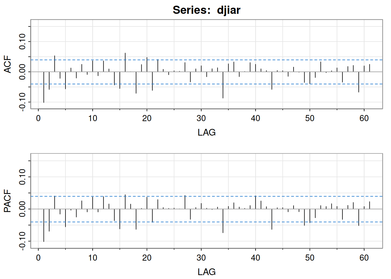
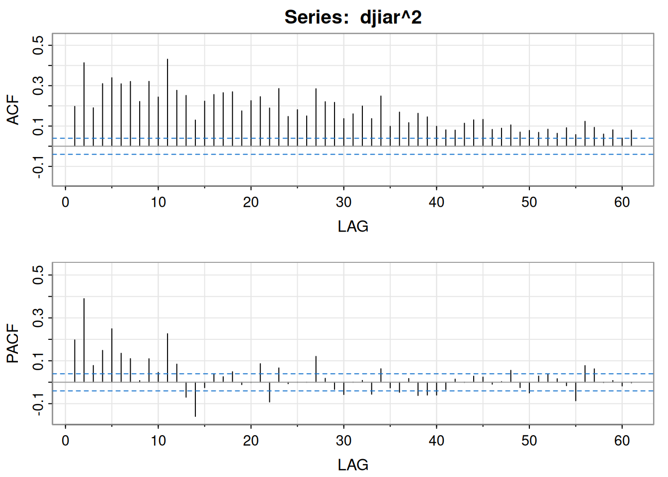
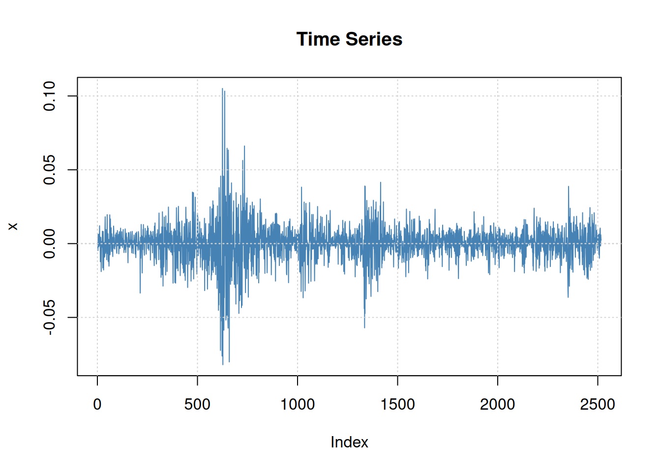
5.2.5.2 Ejemplo: Análisis GARCH del retorno DJIA
En este caso se usa errores t-Student para capturar colas un poco más pesadas(ver Manual fGarch):
library(xts)
Loading required package: zoo
Attaching package: 'zoo'
The following objects are masked from 'package:base':

    as.Date, as.Date.numeric
######################### Warning from 'xts' package ##########################
#                                                                             #
# The dplyr lag() function breaks how base R's lag() function is supposed to  #
# work, which breaks lag(my_xts). Calls to lag(my_xts) that you type or       #
# source() into this session won't work correctly.                            #
#                                                                             #
# Use stats::lag() to make sure you're not using dplyr::lag(), or you can add #
# conflictRules('dplyr', exclude = 'lag') to your .Rprofile to stop           #
# dplyr from breaking base R's lag() function.                                #
#                                                                             #
# Code in packages is not affected. It's protected by R's namespace mechanism #
# Set `options(xts.warn_dplyr_breaks_lag = FALSE)` to suppress this warning.  #
#                                                                             #
###############################################################################
Attaching package: 'xts'
The following objects are masked from 'package:dplyr':

    first, last
djiar =diff(log(djia$Close))[-1]acf2(djiar) # autocorrelación baja (no mostrado)
Modelo de potencia asimétrico ARCH con varianza condicional:
\[
\sigma_t^\delta=\alpha_0+\sum_{j=1}^p \alpha_j\left(\lvert r_{t-j}\rvert-\gamma_j r_{t-j}\right)^\delta
+\sum_{j=1}^q \beta_j \sigma_{t-j}^\delta,
\] Nótese que el modelo es GARCH cuando \(\delta = 2\) y \(\gamma_j = 0\), para \(j \in \{1, \ldots, p\}\). Los parámetros \(\gamma_j\) (\(|\gamma_j| \leq 1\)) son los parámetros de apalancamiento (leverage), que representan una medida de asimetría, y \(\delta > 0\) es el parámetro del término de potencia.
Un valor positivo [negativo] de \(\gamma_j\) significa que los choques negativos [positivos] pasados tienen un impacto más fuerte en la volatilidad condicional actual que los choques positivos [negativos] pasados. Este modelo combina la flexibilidad de un exponente variable con el coeficiente de asimetría para tener en cuenta el efecto de apalancamiento.
Además, para garantizar que \(\sigma_t > 0\), se asume que \(\alpha_0 > 0\), \(\alpha_j \geq 0\) (con al menos un \(\alpha_j > 0\)) y \(\beta_j \geq 0\).
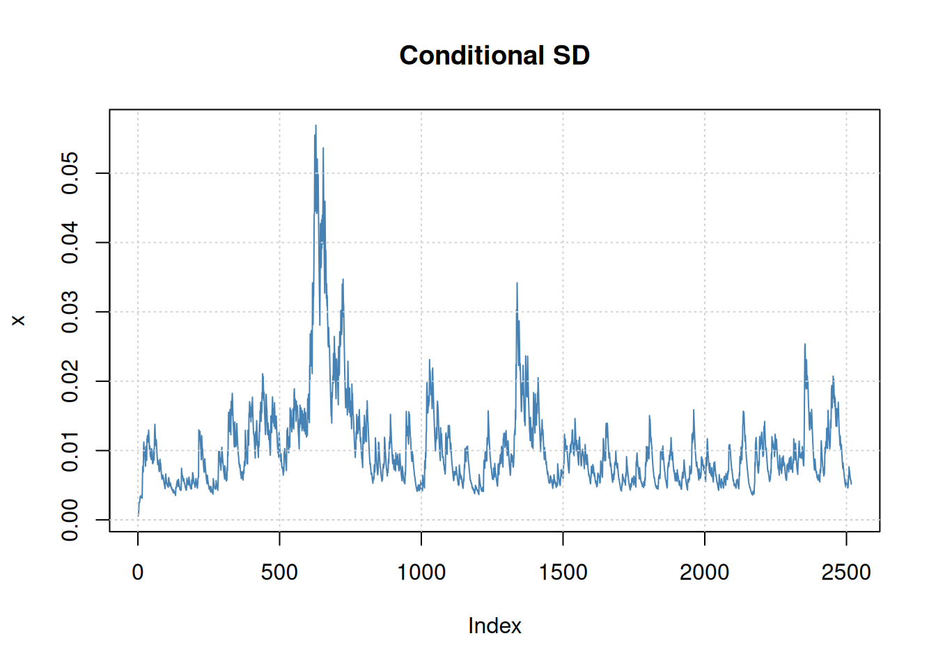
5.2.6.1 Continuación del ejemplo del DJIA:
Siempre con errores t-Student:
library(xts)library(fGarch)summary(djia.ap <-garchFit(~arma(1,0) +aparch(1,1), data = djiar,cond.dist ='std'))
En GARCH, \(\sigma_t^2\) es determinística condicionalmente. El modelo de volatilidad estocástica introduce aleatoriedad: \[
r_t=\sigma_t \epsilon_t \ \Rightarrow\ \log r_t^2=\log \sigma_t^2+\log \epsilon_t^2
\] y la volatilidad latente sigue \[
\log \sigma_{t+1}^2=\phi_0+\phi_1 \log \sigma_t^2+w_t,\quad w_t\sim \text{iid }N(0,\sigma_w^2).
\] El objetivo es estimar \(\phi_0,\phi_1,\sigma_w^2\) y predecir la volatilidad futura.
5.3 Modelos de Umbral (Threshold Models)
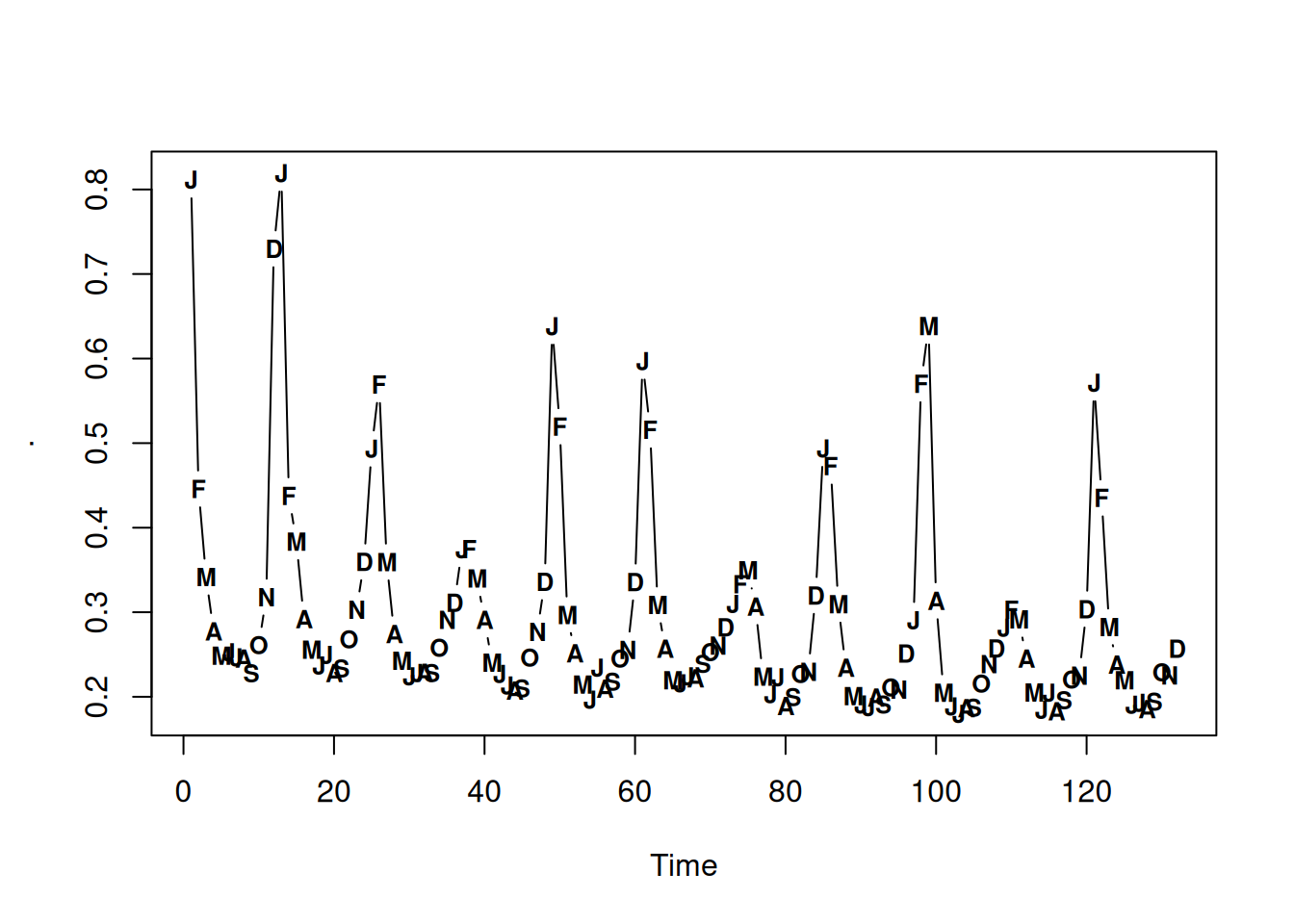
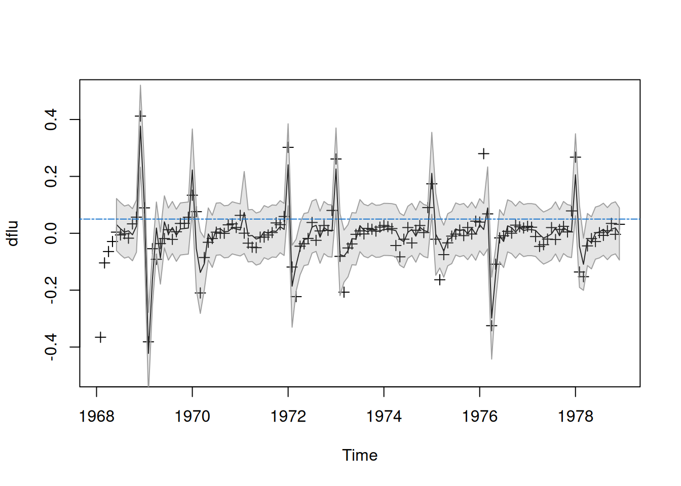
Para una serie temporal estacionaria, la mejor predicción lineal hacia adelante es igual a la mejor predicción lineal hacia atrás. Esto se debe a que la matriz de varianza-covarianza \(\Gamma = {\gamma(i-j)}_{i,j=1}^n\) es simétrica y los procesos gaussianos tienen distribuciones idénticas al invertirse en el tiempo. Sin embargo, muchas series reales no cumplen esta propiedad: por ejemplo, las muertes por influenza aumentan más rápido de lo que disminuyen, mostrando asimetrías y no estacionalidad perfecta.
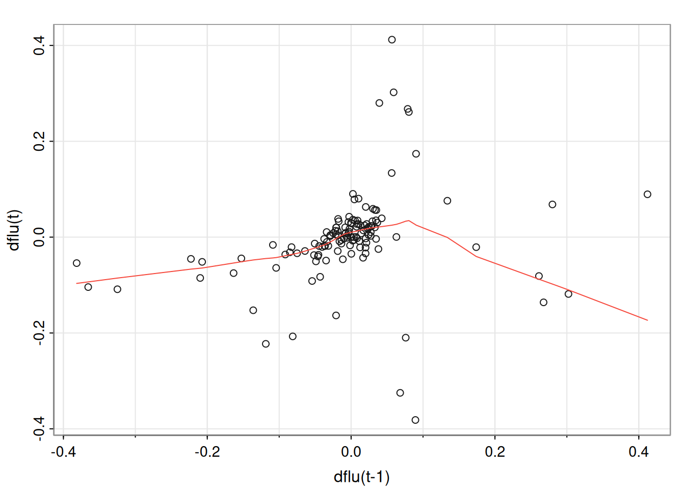
5.3.1 Modelos TARMA (Threshold ARMA)
Una alternativa no lineal es el modelo TARMA (Threshold ARMA), que ajusta modelos lineales locales en distintos regímenes. Un modelo SETARMA (Self-Exciting Threshold ARMA) de \(k\) regímenes se define como:
donde \(w_t^{(j)} \sim \text{iid } N(0, \sigma_j^2)\) para \(j = 1, \ldots, k\), \(d\) es un retardo, y \(r_1 < \cdots < r_{k-1}\) son los umbrales que dividen los regímenes.
Cada régimen corresponde a un modelo ARMA diferente, y las condiciones de estacionariedad e invertibilidad dependen de las propiedades de cada régimen.
Extensiones del modelo
El umbral puede depender de valores pasados del proceso o de variables exógenas. En ese caso, puede sustituirse \(x_{t-d}\) por otra variable \(y_{t-d}\) que represente tales variables.
5.3.1.1 Ejemplo: Modelado de la serie de influenza
Se estudia la serie mensual de muertes por neumonía e influenza, \(\mathrm{flu}_t\), que muestra un leve descenso y una clara no linealidad. Para eliminar la tendencia, se trabaja con las primeras diferencias:
\[
x_t = \mathrm{flu}_t - \mathrm{flu}_{t-1}.
\]
Se observa que \(x_t\) aumenta lentamente y luego puede saltar bruscamente cuando supera aproximadamente 0.05, sugiriendo dos regímenes según \(x_{t-1}\).
Errores estándar: \[
\begin{equation*}
\operatorname{se}\left(\hat{\beta}_{i j}\right)=\sqrt{c_{i i} \hat{\sigma}_{j j}},
\end{equation*}
\] donde \(c_{ii}\) es el elemento (i)-ésimo diagonal de \(\left(\sum z_t z_t'\right)^{-1}\) y \(\hat{\sigma}_{jj}\) el (j)-ésimo diagonal de \(\hat{\Sigma}_w\).
Modelo autoregresivo vectorial de primer orden: \[
\begin{equation*}
x_{t}=\alpha+\Phi x_{t-1}+w_{t},
\end{equation*}
\] con \(\mathrm{E}(w_t w_t')=\Sigma_w\)\(k\times k\) y \(\alpha=(I-\Phi)\mu\) si \(\mathrm{E}(x_t)=\mu\).
Identificación con regresión multivariante: \(y_t=x_t\), \(\mathcal{B}=(\alpha,\Phi)\), \(z_t=(1,x_{t-1})\). Estimación condicional de \(\Sigma_w\):
Extensión ARX (exógenas) de orden (p): \[
\begin{equation*}
x_{t}=\Gamma u_{t}+\sum_{j=1}^{p} \Phi_{j} x_{t-j}+w_{t}. \end{equation*}
\]
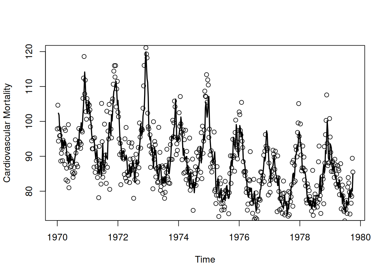
5.4.1.1 Ejemplo (Contaminación, clima y mortalidad)
# Paquete para VARlibrary(vars)
Loading required package: MASS
Attaching package: 'MASS'
The following object is masked from 'package:dplyr':

    select
Loading required package: strucchange
Loading required package: sandwich
Attaching package: 'strucchange'
The following object is masked from 'package:stringr':

    boundary
Loading required package: urca
Loading required package: lmtest
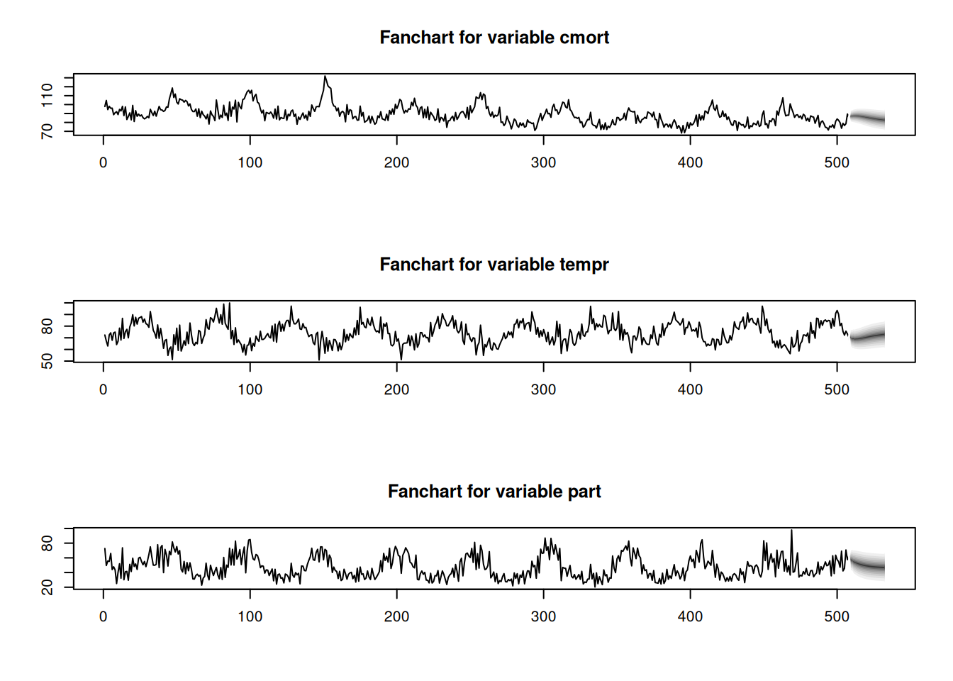
# Matriz de series: mortalidad, temperatura, particuladox <-cbind(cmort, tempr, part)# Ajuste VAR(1) con constante y tendenciasummary(VAR(x, p =1, type ="both"))
VAR Estimation Results:
=========================
Endogenous variables: cmort, tempr, part
Deterministic variables: both
Sample size: 507
Log Likelihood: -5116.02
Roots of the characteristic polynomial:
0.8931 0.4953 0.1444
Call:
VAR(y = x, p = 1, type = "both")


Estimation results for equation cmort:
======================================
cmort = cmort.l1 + tempr.l1 + part.l1 + const + trend

          Estimate Std. Error t value Pr(>|t|)
cmort.l1  0.464824   0.036729  12.656  < 2e-16 ***
tempr.l1 -0.360888   0.032188 -11.212  < 2e-16 ***
part.l1   0.099415   0.019178   5.184 3.16e-07 ***
const    73.227292   4.834004  15.148  < 2e-16 ***
trend    -0.014459   0.001978  -7.308 1.07e-12 ***
---
Signif. codes:  0 '***' 0.001 '**' 0.01 '*' 0.05 '.' 0.1 ' ' 1


Residual standard error: 5.583 on 502 degrees of freedom
Multiple R-Squared: 0.6908, Adjusted R-squared: 0.6883
F-statistic: 280.3 on 4 and 502 DF,  p-value: < 2.2e-16


Estimation results for equation tempr:
======================================
tempr = cmort.l1 + tempr.l1 + part.l1 + const + trend

          Estimate Std. Error t value Pr(>|t|)
cmort.l1 -0.244046   0.042105  -5.796 1.20e-08 ***
tempr.l1  0.486596   0.036899  13.187  < 2e-16 ***
part.l1  -0.127661   0.021985  -5.807 1.13e-08 ***
const    67.585598   5.541550  12.196  < 2e-16 ***
trend    -0.006912   0.002268  -3.048  0.00243 **
---
Signif. codes:  0 '***' 0.001 '**' 0.01 '*' 0.05 '.' 0.1 ' ' 1


Residual standard error: 6.4 on 502 degrees of freedom
Multiple R-Squared: 0.5007, Adjusted R-squared: 0.4967
F-statistic: 125.9 on 4 and 502 DF,  p-value: < 2.2e-16


Estimation results for equation part:
=====================================
part = cmort.l1 + tempr.l1 + part.l1 + const + trend

          Estimate Std. Error t value Pr(>|t|)
cmort.l1 -0.124775   0.079013  -1.579    0.115
tempr.l1 -0.476526   0.069245  -6.882 1.77e-11 ***
part.l1   0.581308   0.041257  14.090  < 2e-16 ***
const    67.463501  10.399163   6.487 2.10e-10 ***
trend    -0.004650   0.004256  -1.093    0.275
---
Signif. codes:  0 '***' 0.001 '**' 0.01 '*' 0.05 '.' 0.1 ' ' 1


Residual standard error: 12.01 on 502 degrees of freedom
Multiple R-Squared: 0.3732, Adjusted R-squared: 0.3683
F-statistic: 74.74 on 4 and 502 DF,  p-value: < 2.2e-16


Covariance matrix of residuals:
       cmort  tempr   part
cmort 31.172  5.975  16.65
tempr  5.975 40.965  42.32
part  16.654 42.323 144.26

Correlation matrix of residuals:
       cmort  tempr   part
cmort 1.0000 0.1672 0.2484
tempr 0.1672 1.0000 0.5506
part  0.2484 0.5506 1.0000
Resultados clave (parciales, en el texto): estimaciones \(\hat{\alpha}, \hat{\beta}, \hat{\Phi}\), \(\hat{\Sigma}_w\) y ecuación de predicción para mortalidad \(\hat{M}_t=73.23-0.014t+0.46M_{t-1}-0.36T_{t-1}+0.10P_{t-1}\) con \(R^2\approx 0.69\).
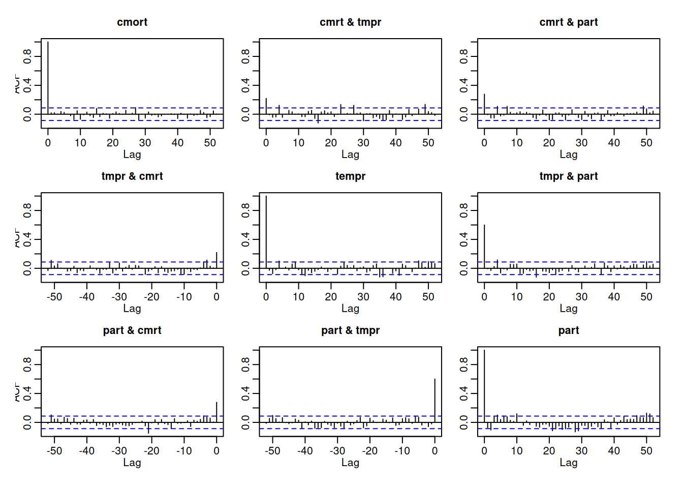
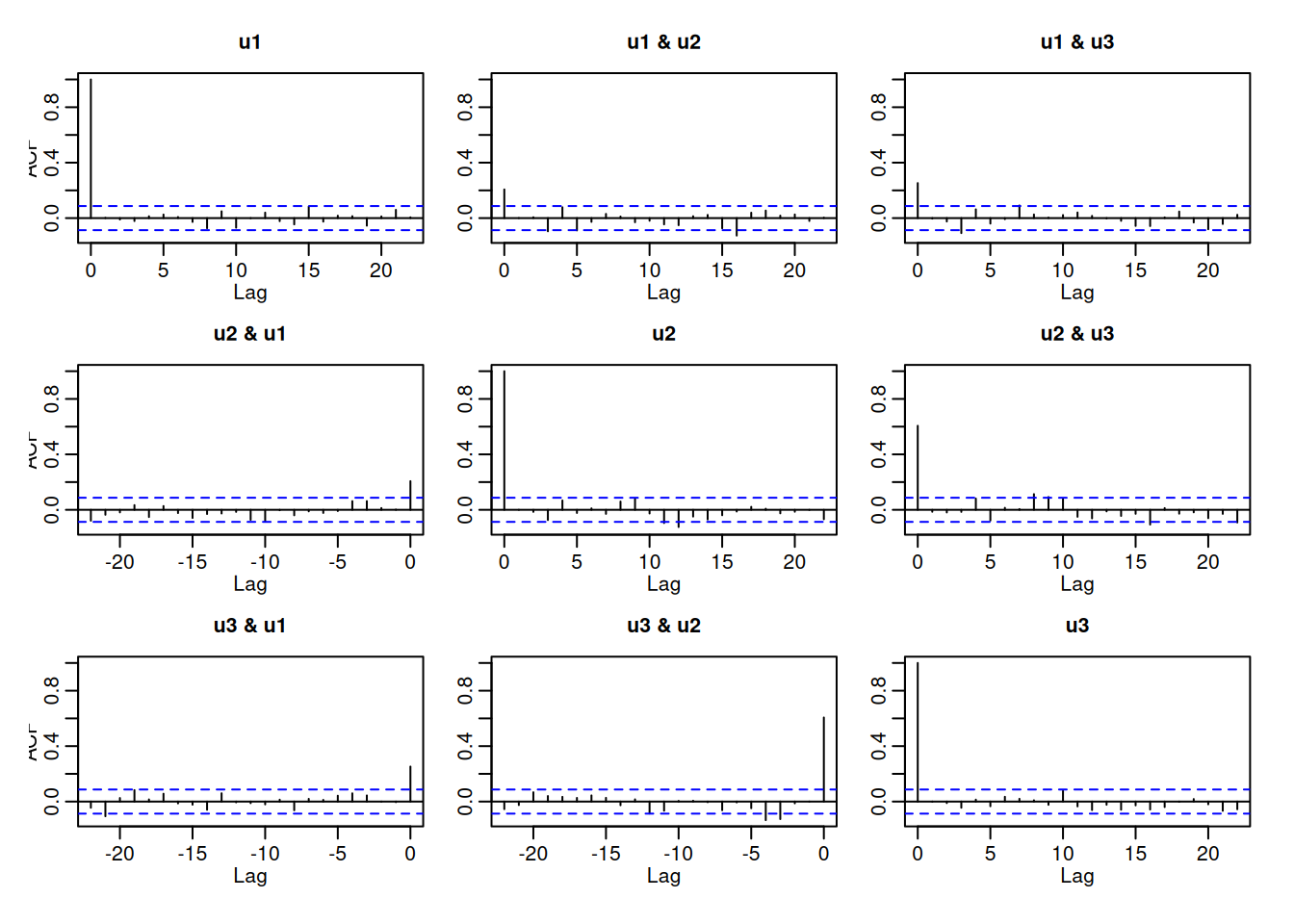
# Diagnóstico: ACFs y prueba Portmanteau ajustadaacf(resid(fit), 52)
serial.test(fit, lags.pt =12, type ="PT.adjusted")
    Portmanteau Test (adjusted)

data:  Residuals of VAR object fit
Chi-squared = 162.35, df = 90, p-value = 4.602e-06
Interpretación: BIC selecciona (p=2) (frente a AIC/FPE/HQ). El diagnóstico multivariante indica que el modelo no captura efectos concurrentes (correlaciones residuales no nulas), por lo que el test Q (equivalente al Ljung-Box univariado) rechaza ruido blanco.
Sea \(\phi=\operatorname{vec}(\Phi_1,\ldots,\Phi_p)\) (vector \(k^2p\times 1\). Entonces, \[
\begin{equation*}
\sqrt{n}(\hat{\phi}-\phi) \sim A N\left(0, \Sigma_{w} \otimes \Gamma_{pp}^{-1}\right),
\end{equation*}
\] donde \(\Gamma_{pp}={\Gamma(i-j)}_{i,j=1}^p\). Errores estándar a partir de \(\hat{\Sigma}_w) y (\hat{\Gamma}_{pp}\).
5.4.5 VARMA y ARMAX multivariados: operadores y condiciones
Causalidad: raíces de \(|\Phi(z)|\) fuera del círculo unitario; Invertibilidad: raíces de \(|\Theta(z)|\) fuera del círculo unitario. Representaciones: \[
x_t=\Psi(B)w_t,\quad \Psi(B)=\sum_{j=0}^\infty \Psi_j B^j,\ \Psi_0=I;
\]\[
w_t=\Pi(B)x_t,\quad \Pi(B)=\sum_{j=0}^\infty \Pi_j B^j,\ \Pi_0=I.
\]
5.4.6 Estructura de autocovarianza
Para modelo causal ARMA((p,q)) ((h)): \[
\begin{equation*}
\Gamma(h)=\sum_{j=0}^{\infty} \Psi_{j+h} \Sigma_{w} \Psi_{j}^{\prime},
\end{equation*}
\] Para MA((q)): \[
\begin{equation*}
\Gamma(h)=\sum_{j=0}^{q-h} \Theta_{j+h} \Sigma_{w} \Theta_{j}^{\prime}, \quad \Theta_0=I,
\end{equation*}
\] y \(\Gamma(h)=0\) para (h>q).
5.4.7 Algoritmo de Spliid para VARMA (estimación rápida)
Modelo general con media no nula: \[
\begin{equation*}
x_{t}=\alpha+\Phi_{1} x_{t-1}+\cdots+\Phi_{p} x_{t-p}+w_{t}+\Theta_{1} w_{t-1}+\cdots+\Theta_{q} w_{t-q}.
\end{equation*}
\] Si \(\mu=\mathrm{E}x_t\), entonces \(\alpha=(I-\Phi_1-\cdots-\Phi_p)\mu\).
Si \(w_{t-1},\dots,w_{t-q}\) fueran observables, el modelo anterior se puede reescribir como regresión multivariante: \[
\begin{equation*}
x_{t}=\mathcal{B} z_{t}+w_{t},
\end{equation*}
\]\[
\begin{equation*}
z_{t}=\left(1, x_{t-1}^{\prime}, \ldots, x_{t-p}^{\prime}, w_{t-1}^{\prime}, \ldots, w_{t-q}^{\prime}\right)^{\prime},
\end{equation*}
\]\[
\begin{equation*}
\mathcal{B}=\left[\alpha, \Phi_{1}, \ldots, \Phi_{p}, \Theta_{1}, \ldots, \Theta_{q}\right].
\end{equation*}
\]
Actualización de innovaciones (dadas \(\mathcal{B}_0\)):
Los nuevos valores de \(w_t\) se incluyen en las covariables \(z_t\) y se vuelve a estimar \(\mathcal{B}\) hasta convergencia (no necesariamente MLE, pero cercano y útil como inicialización para métodos de espacio de estados).
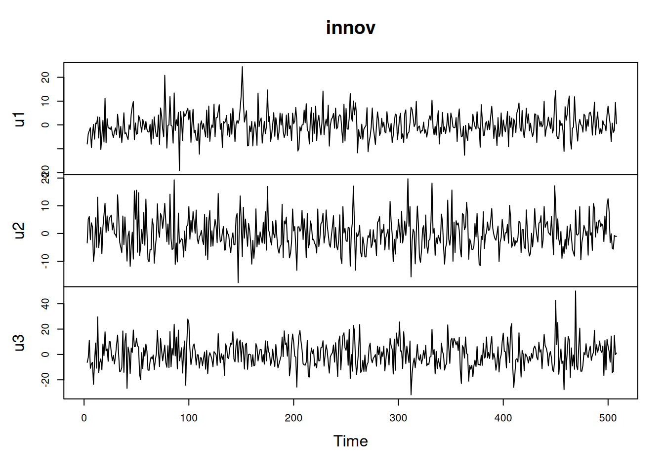
5.4.7.1 Ejemplo (Algoritmo de Spliid con marima)
library(marima)# Definición del modelo VARMA(2,1)model <-define.model(kvar =3, ar =c(1, 2), ma =c(1))arp <- model$ar.pattern; map <- model$ma.pattern# Detrendeo de mortalidad (cmort) y armado de matriz de datoscmort.d <-resid(detr <-lm(cmort ~time(cmort), na.action =NULL))xdata <-matrix(cbind(cmort.d, tempr, part), ncol =3) # quitar atributos ts# Ajuste VARMA con penalizaciónfit <-marima(xdata, ar.pattern = arp, ma.pattern = map, means =c(0, 1, 1),penalty =1)
All cases in data,  1  to  508  accepted for completeness.
508 3  = MARIMA - dimension of data
# Innovaciones y diagnóstico (no mostrado)innov <-t(resid(fit)); plot.ts(innov); acf(innov, na.action = na.pass)